Study of the Reliability of Questionnaire-Based Diagnosis of Socionic Variables
Study of the Reliability of Questionnaire-Based Diagnosis of Socionic Variables
V. L. Talanov
St. Petersburg, June 2017
Contents
- Preface for Socionists
- Summary
- Introduction
- Cronbach’s Method for Calculating Reliability (Calculation of Cronbach’s “Alpha” Coefficient for the Socionic Scales Used by the Questionnaires). Cronbach’s Alpha – Theoretical Part
- Calculation of Cronbach’s Alpha (Reliability) Separately for the Scales of the Main Socionic Indicators in V. L. Talanov’s Socionic Diagnostic Questionnaires
- Reliability of All Individual Socionic Indicators Measured by V. L. Talanov’s Psychodiagnostic Questionnaires Using the Split-Half Method (“Method of Autonomous Parts”)
- Individual Indicators of Psychodiagnostic Test Reliability for a Specific Individual Respondent
- Agreement Between the Psychotype from Self-Typing and the Psychotype from Questionnaire Diagnosis as a Function of Respondents’ Individual Test-Reliability Indicators
- Agreement Between the Psychotype from Self-Typing and the Psychotype from Questionnaire Diagnosis as a Function of Respondents’ Sex, Age, and Socionics Experience
- Differences in Agreement and Type-Profile Reliability Indicators Depending on the Declared Psychotype – Facts and Analysis of Causes. Main Influencing Factors
- First Factor - Different Competence in Psychological Self-Assessment Among Representatives of Different Psychotypes When Reflecting and Understanding Their Own Psychological Properties in Comparison with Other People
- Second Factor - Fashionable and Unfashionable Types
- Third Factor - Diffusion of Errors from Frequent Types to Rare Types
- Fourth and Final Factor Affecting Between-Type Differences in Mean Diagnostic Agreement – the Factor of Mean Distance from the TIM’s Location in Multidimensional Psychological Space to the Locations of Other TIMs (Factor of the TIM’s Mean Remoteness from the Other 15 TIMs)
- Calculation and Comparison of the Mean Probabilities of Identifying the True Type in Self-Typing and in MOLTI Questionnaire Diagnosis
- Intercorrelations of Within-Test Indicators Related to Test Reliability
- Test-Retest Reliability Assessment of MOLTI-Series Questionnaires Using Questionnaires of the Same Form
- Conclusions
- Recommended Articles
- Conditions for Reproduction of the Article
- Contacts
The article contains 10 figures and 22 tables.
1. Preface for Socionists
The article provides a detailed answer to all questions that have arisen, or could arise, in connection with the reliability of methods of socionic diagnosis using questionnaires. Everyone for whom these questions have not yet “cooled off,” as well as those who work professionally with questionnaire-based diagnosis, is advised to examine this article in as much detail as possible. In places it contains a great deal of mathematics – but this is unavoidable.
2. Summary
The article provides a detailed and extensive analysis of various issues of reliability in the measurement of socionic variables by socionic diagnostic questionnaires. V. L. Talanov’s socionic diagnostic questionnaires are used as the material for the analysis, but most of the conclusions, formulas, and tabular data resulting from this examination will be useful not only to the narrow circle of professional socionists, but also to a much broader range of specialists engaged in the development of any psychodiagnostic questionnaires (not necessarily socionic ones) or in the interpretation of their results.
The article shows how to apply Cronbach’s method to assess the reliability of questionnaire scales based on measuring correlations or covariances between respondents’ answers and diagnostic vectors. Special parameters f and Z are developed for predicting the agreement of two independent discrete diagnoses in a sample of respondents who in reality are distributed continuously between the reference points of the diagnoses. Using parameter f (Section 8 of the article), it is shown that the psychological space between discrete psychotypes is indeed continuously populated by respondents in the sample. It is shown that a respondent’s simultaneous proximity to two, or even three, types is not uncommon and is the cause of an obligatory and calculable reduction in the agreement of independent diagnoses even when respondents’ type profiles have high reliability and substantial height. Specifically with regard to Talanov’s socionic diagnostic questionnaires (including the MOLTI-series questionnaires), it is shown that the socionic indicators measured by them satisfy all requirements of the reliability criteria (Cronbach’s alpha, correlations of equivalent parts, and retest correlations) imposed on professional psychodiagnostic questionnaires. From the standpoint of testing-reliability requirements, quantitative criteria for questionnaire items are developed that make it possible to perform a mathematically meaningful selection of items for the diagnostic scales of any psychological questionnaires. For the diagnosis of socionic types, all factors leading to unequal accumulation of errors (and ultimately to different agreement) in different type groups of subjects are analyzed in detail. Cases in which these type groups are formed from self-typing results and cases in which they are formed from questionnaire-typing results are considered separately. A method is shown for separately calculating the probabilities of correctly identifying the true type in self-typing and in questionnaire diagnosis, based on the agreement of the corresponding diagnoses and on the variance of mean agreement across the 16 psychotype groups (calculated separately for type groups formed by self-typing and by questionnaire diagnosis). For self-typing, the calculation yields a sample-average probability of correctly identifying the true type of about 63%, whereas for diagnosis using MOLTI questionnaires with 220 diagnostic questions it is about 83% on average across the sample.
3. Introduction
V. L. Talanov’s socionic diagnostic questionnaires (whose reliability is analyzed in the present article) are self-learning, with a recurrent training procedure and with initial reliance on subjects’ self-typing (on the psychotypes declared by respondents on the basis of their self-assessment in parallel with questionnaire typing).
First stage of questionnaire training. Suppose that, for a certain questionnaire item, we have the answers of a sufficiently large number of subjects who have declared their psychotype on the basis of self-assessment. Within the group for each declared psychotype, we can calculate the mean response score for that item. Usually, this procedure is performed on subjects’ responses that have first been cleared of the influence of social dissimulation and individual response-style characteristics (such as preferences for high or low ratings) and then finally normalized (during normalization, raw response scores from 1 to 5 are transformed into normalized item scores with a sample mean of zero and a sample standard deviation of one). The responses of different subjects who declared the same type are taken into account with different weights when calculating type-group mean scores. The weighting function used is optimal (as determined from mathematical experiments) and reflects both the subject’s confidence in the declared type and the subject’s socionics competence, which depends on the length of their familiarity with socionics.
Given that, as calculations show, the mean accuracy of self-typing among respondents who declare their type is approximately 62%-66%, this quality of formation of the training type samples is entirely sufficient to obtain quite reliable type profiles for each questionnaire item examined. It is true that this procedure contains certain “pitfalls” - for example, first, psychotypes that are rare in the sample become contaminated by errors (false alarms) originating from psychotypes that are more frequent in the sample (the so-called diffusion of errors from more frequent types toward rarer ones). Second, because people are continuously distributed in psychological space between psychotypes, the mean coordinate values of psychotypes that are rare in the sample also become shifted toward psychotypes that are more frequent and similar in their properties (the “statistical slope” effect). Third, there is also the effect of “social fashionability,” that is, greater or lesser social popularity of choosing each psychotype in self-typing. To increase the precision and adequacy of diagnosis, all of these systematic errors must be taken into account and corrected. Fortunately, in practice all these undesirable effects are modeled mathematically quite easily (or at least reliably), and therefore can be fully compensated computationally on the basis of the resulting mathematical models (the mechanisms for correcting them are among the subjects addressed in the present article). As a result, on the basis of the training sample we ultimately obtain an objective and practically unbiased picture of the normalized responses to each questionnaire item of interest, averaged within each training type group; that is, for each questionnaire item we obtain a set of 16 algebraic numbers – the type profile of that questionnaire item.
Second stage of questionnaire training. If we have a questionnaire consisting, say, of 300 items, for each of which a type profile has been calculated in the training sample, we effectively have 16 diagnostic vectors (one vector for each TIM), each consisting of 300 algebraic numbers, “reference responses” – the normalized responses of respondents in the training sample, averaged by type group. By comparing a new subject’s vector of normalized answers to these same 300 questions with the 16 vectors of reference responses (specifically, by measuring the linear correlation between the subject’s answers and each of the 16 diagnostic vectors), we obtain for each subject a set of 16 numbers characterizing the proximity of that subject’s responses to each of the 16 “standard” psychotypes. The psychotype for which the highest correlation coefficient with the subject’s responses is obtained is taken to be the subject’s true psychotype. In new samples (which did not previously participate in the training procedure used to obtain the primary diagnostic coefficients), the agreement of these newly diagnosed psychotypes with the psychotypes declared by the subjects themselves (that is, with their self-typed psychotypes) averages, across different questionnaires, from 55% to 61%. Detailed mathematical calculation shows that the accuracy of the newly diagnosed psychotypes is substantially higher than that of the psychotypes declared by self-typing (this issue is also examined in the present article). If the latter, as indicated above, is approximately 62%-66%, the former gives an accuracy of assignment to the true psychotype (that is, the objectively closest standard psychotype) of 80% to 95% (again varying across questionnaires, depending on their length and item selection). The newly obtained type diagnoses (which are more accurate and, moreover, now available for all subjects rather than only the subset who declared their type) form the training sample of the next, second level. On this sample, mean responses by psychotype to each questionnaire item are again calculated, producing new, refined, and more contrastive (less noisy) vectors of reference responses for each psychotype. The responses of different subjects, even those belonging to the same type, are again taken into account with different weights during this within-type averaging – but this time in proportion to Fisher’s function of the linear correlation coefficient between the reference responses of the corresponding standard psychotype, to which the subject is closest, and the subject’s vector of normalized responses. The resulting diagnostic coefficients of the questionnaire items (that is, their numerical type profiles) can then be used as final coefficients.
Table 1. Conversion of type profiles into trait profiles (for any type profile, the corresponding value of any trait loading is obtained by taking the scalar product of the row of 16 numerical loadings of the corresponding type profile and the row of algebraic coefficients for the trait of interest in the present table). All numbers in the table have an absolute value of 1/16.
| ILE | LII | SEI | ESE | SLE | LSI | IEI | EIE | SEE | ESI | ILI | LIE | IEE | EII | SLI | LSE | |
|---|---|---|---|---|---|---|---|---|---|---|---|---|---|---|---|---|
| Extraversion | 0,0625 | -0,0625 | -0,0625 | 0,0625 | 0,0625 | -0,0625 | -0,0625 | 0,0625 | 0,0625 | -0,0625 | -0,0625 | 0,0625 | 0,0625 | -0,0625 | -0,0625 | 0,0625 |
| Irrationality | 0,0625 | -0,0625 | 0,0625 | -0,0625 | 0,0625 | -0,0625 | 0,0625 | -0,0625 | 0,0625 | -0,0625 | 0,0625 | -0,0625 | 0,0625 | -0,0625 | 0,0625 | -0,0625 |
| Static | 0,0625 | 0,0625 | -0,0625 | -0,0625 | 0,0625 | 0,0625 | -0,0625 | -0,0625 | 0,0625 | 0,0625 | -0,0625 | -0,0625 | 0,0625 | 0,0625 | -0,0625 | -0,0625 |
| Intuition | 0,0625 | 0,0625 | -0,0625 | -0,0625 | -0,0625 | -0,0625 | 0,0625 | 0,0625 | -0,0625 | -0,0625 | 0,0625 | 0,0625 | 0,0625 | 0,0625 | -0,0625 | -0,0625 |
| Judicious (Peripheral) | 0,0625 | 0,0625 | 0,0625 | 0,0625 | -0,0625 | -0,0625 | -0,0625 | -0,0625 | -0,0625 | -0,0625 | -0,0625 | -0,0625 | 0,0625 | 0,0625 | 0,0625 | 0,0625 |
| Tactical | 0,0625 | -0,0625 | -0,0625 | 0,0625 | -0,0625 | 0,0625 | 0,0625 | -0,0625 | -0,0625 | 0,0625 | 0,0625 | -0,0625 | 0,0625 | -0,0625 | -0,0625 | 0,0625 |
| Carefree | 0,0625 | -0,0625 | 0,0625 | -0,0625 | -0,0625 | 0,0625 | -0,0625 | 0,0625 | -0,0625 | 0,0625 | -0,0625 | 0,0625 | 0,0625 | -0,0625 | 0,0625 | -0,0625 |
| Logic | 0,0625 | 0,0625 | -0,0625 | -0,0625 | 0,0625 | 0,0625 | -0,0625 | -0,0625 | -0,0625 | -0,0625 | 0,0625 | 0,0625 | -0,0625 | -0,0625 | 0,0625 | 0,0625 |
| Merry (Ascending) | 0,0625 | 0,0625 | 0,0625 | 0,0625 | 0,0625 | 0,0625 | 0,0625 | 0,0625 | -0,0625 | -0,0625 | -0,0625 | -0,0625 | -0,0625 | -0,0625 | -0,0625 | -0,0625 |
| Constructivist | 0,0625 | -0,0625 | -0,0625 | 0,0625 | 0,0625 | -0,0625 | -0,0625 | 0,0625 | -0,0625 | 0,0625 | 0,0625 | -0,0625 | -0,0625 | 0,0625 | 0,0625 | -0,0625 |
| Yielding | 0,0625 | -0,0625 | 0,0625 | -0,0625 | 0,0625 | -0,0625 | 0,0625 | -0,0625 | -0,0625 | 0,0625 | -0,0625 | 0,0625 | -0,0625 | 0,0625 | -0,0625 | 0,0625 |
| Questimity | 0,0625 | 0,0625 | -0,0625 | -0,0625 | -0,0625 | -0,0625 | 0,0625 | 0,0625 | 0,0625 | 0,0625 | -0,0625 | -0,0625 | -0,0625 | -0,0625 | 0,0625 | 0,0625 |
| Democratic (Individualist) | 0,0625 | 0,0625 | 0,0625 | 0,0625 | -0,0625 | -0,0625 | -0,0625 | -0,0625 | 0,0625 | 0,0625 | 0,0625 | 0,0625 | -0,0625 | -0,0625 | -0,0625 | -0,0625 |
| Positivist | 0,0625 | -0,0625 | -0,0625 | 0,0625 | -0,0625 | 0,0625 | 0,0625 | -0,0625 | 0,0625 | -0,0625 | -0,0625 | 0,0625 | -0,0625 | 0,0625 | 0,0625 | -0,0625 |
| Process (Rightist) | 0,0625 | -0,0625 | 0,0625 | -0,0625 | -0,0625 | 0,0625 | -0,0625 | 0,0625 | 0,0625 | -0,0625 | 0,0625 | -0,0625 | -0,0625 | 0,0625 | -0,0625 | 0,0625 |
Table 2. Conversion of trait profiles into functional profiles (the magnitude of each function is obtained by taking the scalar product of the row of 15 trait loadings and the row of coefficients from this table for the function of interest)
| Extraversion | Irrationality | Static | Intuition | Judicious (Peripheral) | Tactical | Carefree | Logic | Merry (Ascending) | Constructivist | Yielding | Questimity | Democratic (Individualist) | Positivist | Process (Rightist) | |
|---|---|---|---|---|---|---|---|---|---|---|---|---|---|---|---|
| Ni | -1 | 1,5 | -1 | 3 | -3 | 0 | 0 | 0 | 0 | 0 | 0 | 0 | 0 | 0 | 0 |
| Ne | 1 | 1,5 | 1 | 3 | 3 | 0 | 0 | 0 | 0 | 0 | 0 | 0 | 0 | 0 | 0 |
| Si | -1 | 1,5 | -1 | -3 | 3 | 0 | 0 | 0 | 0 | 0 | 0 | 0 | 0 | 0 | 0 |
| Se | 1 | 1,5 | 1 | -3 | -3 | 0 | 0 | 0 | 0 | 0 | 0 | 0 | 0 | 0 | 0 |
| Ti | -1 | -0,75 | 1 | 0 | 0 | 0 | 0 | 3 | 3 | 0 | 0 | 0 | 0 | 0 | 0 |
| Te | 1 | -0,75 | -1 | 0 | 0 | 0 | 0 | 3 | -3 | 0 | 0 | 0 | 0 | 0 | 0 |
| Fi | -1 | -0,75 | 1 | 0 | 0 | 0 | 0 | -3 | -3 | 0 | 0 | 0 | 0 | 0 | 0 |
| Fe | 1 | -0,75 | -1 | 0 | 0 | 0 | 0 | -3 | 3 | 0 | 0 | 0 | 0 | 0 | 0 |
| Qi | -1 | -0,75 | 1 | 0 | 0 | 0 | 0 | 0 | 0 | 0 | 0 | 3 | 3 | 0 | 0 |
| Qe | 1 | -0,75 | -1 | 0 | 0 | 0 | 0 | 0 | 0 | 0 | 0 | 3 | -3 | 0 | 0 |
| Di | -1 | -0,75 | 1 | 0 | 0 | 0 | 0 | 0 | 0 | 0 | 0 | -3 | -3 | 0 | 0 |
| De | 1 | -0,75 | -1 | 0 | 0 | 0 | 0 | 0 | 0 | 0 | 0 | -3 | 3 | 0 | 0 |
Table 3. Reverse conversion of trait profiles into type profiles (the loading of each TIM in the type profile is obtained by taking the scalar product of the row of 15 trait loadings and the row of coefficients in the table corresponding to the TIM of interest)
| Extraversion | Irrationality | Static | Intuition | Judicious (Peripheral) | Tactical | Carefree | Logic | Merry (Ascending) | Constructivist | Yielding | Questimity | Democratic (Individualist) | Positivist | Process (Rightist) | |
|---|---|---|---|---|---|---|---|---|---|---|---|---|---|---|---|
| ILE | 1 | 1 | 1 | 1 | 1 | 1 | 1 | 1 | 1 | 1 | 1 | 1 | 1 | 1 | 1 |
| LII | -1 | -1 | 1 | 1 | 1 | -1 | -1 | 1 | 1 | -1 | -1 | 1 | 1 | -1 | -1 |
| SEI | -1 | 1 | -1 | -1 | 1 | -1 | 1 | -1 | 1 | -1 | 1 | -1 | 1 | -1 | 1 |
| ESE | 1 | -1 | -1 | -1 | 1 | 1 | -1 | -1 | 1 | 1 | -1 | -1 | 1 | 1 | -1 |
| SLE | 1 | 1 | 1 | -1 | -1 | -1 | -1 | 1 | 1 | 1 | 1 | -1 | -1 | -1 | -1 |
| LSI | -1 | -1 | 1 | -1 | -1 | 1 | 1 | 1 | 1 | -1 | -1 | -1 | -1 | 1 | 1 |
| IEI | -1 | 1 | -1 | 1 | -1 | 1 | -1 | -1 | 1 | -1 | 1 | 1 | -1 | 1 | -1 |
| EIE | 1 | -1 | -1 | 1 | -1 | -1 | 1 | -1 | 1 | 1 | -1 | 1 | -1 | -1 | 1 |
| SEE | 1 | 1 | 1 | -1 | -1 | -1 | -1 | -1 | -1 | -1 | -1 | 1 | 1 | 1 | 1 |
| ESI | -1 | -1 | 1 | -1 | -1 | 1 | 1 | -1 | -1 | 1 | 1 | 1 | 1 | -1 | -1 |
| ILI | -1 | 1 | -1 | 1 | -1 | 1 | -1 | 1 | -1 | 1 | -1 | -1 | 1 | -1 | 1 |
| LIE | 1 | -1 | -1 | 1 | -1 | -1 | 1 | 1 | -1 | -1 | 1 | -1 | 1 | 1 | -1 |
| IEE | 1 | 1 | 1 | 1 | 1 | 1 | 1 | -1 | -1 | -1 | -1 | -1 | -1 | -1 | -1 |
| EII | -1 | -1 | 1 | 1 | 1 | -1 | -1 | -1 | -1 | 1 | 1 | -1 | -1 | 1 | 1 |
| SLI | -1 | 1 | -1 | -1 | 1 | -1 | 1 | 1 | -1 | 1 | -1 | 1 | -1 | 1 | -1 |
| LSE | 1 | -1 | -1 | -1 | 1 | 1 | -1 | 1 | -1 | -1 | 1 | 1 | -1 | -1 | 1 |
4. Cronbach’s Method for Calculating Reliability (Calculation of Cronbach’s “Alpha” Coefficient for the Socionic Scales Used by the Questionnaires). Cronbach’s Alpha – Theoretical Part
In Talanov’s questionnaires, the diagnostic procedure used to calculate any socionic scales is the computation of linear correlation coefficients between, on the one hand, vectors of diagnostic coefficients and, on the other hand, the respondent’s vector of answers to the corresponding diagnostic questions in the questionnaire (before the correlations are calculated, the answers of all subjects in the sample to each questionnaire item are first corrected for social dissimulation and for the individual response-style characteristics of each respondent; at the end of this preliminary procedure they are then normalized across the entire sample of respondents so that the answers to each questionnaire item have a sample mean of zero and a sample standard deviation of one).
According to its mathematical definition, the linear correlation coefficient calculated as the indicator of each socionic scale is proportional to the scalar product of two vectors: the respondent’s vector of normalized answers (answers cleared of some nonsocionic artifacts) and the vector of previously known diagnostic coefficients corresponding to the same questions. In other words, the final indicator of each socionic scale calculated for a respondent is proportional to the algebraic sum of all of the respondent’s answers to the diagnostic questionnaire questions, with these normalized response scores being multiplied element by element by the corresponding diagnostic coefficients when summed. This proportionality of correlations to weighted sums makes it possible to obtain an exact quantitative estimate of the reliability of each scale calculated in this way using Cronbach’s method, which Lee Cronbach specifically developed for such cases.
Let N be the number of diagnostic questions in the questionnaire; M the number of respondents examined (sample size);
{bi} – the vector of each respondent’s answers to N diagnostic questions (with the answers to each individual question normalized across the sample of all M respondents);
{ci} – the vector of diagnostic coefficients for the sequence of N diagnostic questions;
{bi × ci} – for each respondent, the vector of their answers to all N questions, with the answers multiplied by the corresponding diagnostic coefficients.
F = ∑1N(bi × ci)
– the calculated value of the socionic scale, equal to the weighted sum of products (answers multiplied by diagnostic coefficients), that is, the algebraic sum of all N elements of the vector {bi × ci}. When socionic scales are calculated from correlations, the value F must additionally be multiplied at the end by a certain constant, but when assessing measurement reliability we will ignore this multiplication, since multiplication by a constant does not affect the calculated statistical reliability of the measured quantity. Thus, the calculation of the reliability of linear correlations can be replaced in a completely equivalent manner by the clearer and simpler calculation of the reliability of the weighted sums F, which is what we will do throughout the remainder of this section.
Si – the standard deviation of the quantity bi × ci in the sample of M subjects (where bi × ci denotes respondents’ answers to the i-th questionnaire question multiplied by the corresponding diagnostic coefficient);
Di = Si2 – the variance of the quantity bi × ci in the sample of M subjects;
SF – the standard deviation of the scale quantity F defined above in the sample of M subjects;
DF = SF2 – the variance of the scale quantity F in the sample of M subjects.
DN = ∑1NDi
– the sum of the sample variances Di across all N diagnostic questions in the questionnaire.
According to classical test theory, the reliability of test results (that is, reliability) can be expressed as the ratio of the variance of the true score to the variance of the total score. The variance of the total score, in turn, equals the sum of error variance and true-score variance. When error variance in the total obtained result is zero, this ratio equals 1. When, by contrast, true-score variance in the total obtained result equals zero, this ratio expressing reliability becomes zero.
DF(question scale of N questions) = Dtruth + Drandom noise
A (reliability) = Dtruth/(Dtruth + Drandom noise) = (DF - Drandom noise)/DF
It can be shown that, in the most general case, the required ratio is equal to:
A= N/(N-1)*(DF-DN)/DF
This formula derived by Lee Cronbach, characterizing the reliability of any questionnaire-test scale consisting of N questions, is called Cronbach’s “alpha” coefficient, or, more briefly, “Cronbach’s alpha,” or simply the “test reliability coefficient.” Coefficient A takes values from 0 (minimum) to 1 (maximum). The higher A is, the higher the measurement reliability of the scale. In psychology, it is generally accepted that for professional diagnostic questionnaire scales A should be approximately 0,9 or higher.
If R is the linear correlation between independently known TRUE VALUES OF THE TRAIT and the values of scale F that model it (with F composed of the sum of the questions), then R*R=R^2=A (this is a well-known result proved in mathematical statistics).
For a scale consisting of N questionnaire questions to have A=0 (the case of complete unreliability, when there is nothing underlying the scale and it measures no entity), it is sufficient either for all elements of the scale bi*ci to have zero mutual correlations (that is, to be strictly independent variables), or for their mutual correlation to be strictly “noise-like,” that is, for half of the correlations in their intercorrelation matrix to have a positive sign and the other half a negative sign, with their sum being zero.
For a scale consisting of N questionnaire questions to have A=1 (the case of complete, 100% reliability, in which all questions of the scale are strictly aimed at measuring the same entity and all questions do so without random error), all mutual correlations in the intercorrelation matrix of the variables bi*ci must be exactly equal to one. It turns out, however, that even if all correlations in this intercorrelation matrix are positive but quite moderate in absolute magnitude (that is, far from one, for example all equal to 0,2), simply increasing the number of questions in the scale can also bring Cronbach’s reliability coefficient arbitrarily close to the desired value of one.
To make it clearer why this occurs, and how Cronbach’s formula works in general, let us consider the simplest case in which all Si are identical for all N questions and equal to one another (this is possible if all questions have diagnostic coefficients that are equal in absolute magnitude), in which case DN=N*Di= N*Si*Si.
If all questions of the scale have zero correlation with one another (absolutely independent variables, which should result in zero reliability for the scale), then when moving from the individual questions to the scale constructed from them, it turns out that the variances of the answers to these questions are added: DF=N*Di= DN=N^0*DN
Then A = N/(N-1)*(DF-DN)/DF = N/(N-1)*( N*Di - N*Di)/ N*Di = 0
If all questions of the scale have a correlation of one with one another (identical variables, which should ultimately result in unit reliability for the scale), then when moving from the individual questions to the scale constructed from them, it turns out that not the variances but the standard deviations of the answers to these questions are added: SF=N*Si. As for the variance of F, DF= SF*SF = (N*Si)*(N*Si) =N^2* Si^2= N*(N* Si^2)= N*DN=N^1*DN
Then A = N/(N-1)*(DF-DN)/DF = N/(N-1)*( N*DN - DN)/ N*DN = N/(N-1)*( N*DN - DN)/ N*DN= N/(N-1)*(N-1)/N =1
In the intermediate case, when the questions of the scale are correlated with one another with a linear correlation coefficient greater than zero but less than one, we obtain:
DF = Na *DN = N^a*DN (where 0<a<1);
A = N/(N-1)*(DF-DN)/DF = N/(N-1)*( N^a*DN - DN)/ N^a*DN = N/(N-1)*(1-1/N^a)
For any nonzero positive correlation between the questions of the scale that is less than one, and the corresponding positive value of parameter a (also lying between 0 and 1), as N increases the value of indicator A expressed by the last formula will also increase, tending toward 1.
For professional psychological tests, it is generally accepted that the reliability indicator A for their scales should be approximately 0,9 (not lower), that is, the variance of a scale empirically measured by a questionnaire should contain at least 90% of the variance of the true quantity that the scale is intended to measure.
It is not difficult to calculate, for different values of parameter a, the number of questions that the scale must contain for this purpose.
N/(N-1)*(1-1/N^a)=0,9
Solutions of this equation (with respect to finding the required number of questions N, where N>1, to achieve reliability A=0,9) for various values of parameter a (0<a<1) are given in Table 4:
Table 4
| a | N | Cronbach’s A |
|---|---|---|
| 0,05 | 1E+20 | 0,90000 |
| 0,10 | 1E+10 | 0,90000 |
| 0,15 | 4641712 | 0,90000 |
| 0,20 | 99956 | 0,90000 |
| 0,25 | 9964 | 0,90000 |
| 0,30 | 2124 | 0,90000 |
| 0,35 | 694 | 0,90002 |
| 0,40 | 294 | 0,90010 |
| 0,45 | 147 | 0,90027 |
| 0,50 | 81 | 0,90000 |
| 0,55 | 49 | 0,90079 |
| 0,60 | 30 | 0,90007 |
| 0,65 | 20 | 0,90245 |
| 0,70 | 13 | 0,90345 |
| 0,75 | 8 | 0,90260 |
| 0,80 | 5 | 0,90507 |
| 0,85 | 3 | 0,91043 |
| 0,90 | 2 | 0,92823 |
| 0,95 | 2 | 0,96474 |
The table shows that the number of questionnaire-scale questions required to ensure 90% reliability increases very rapidly as parameter a decreases, and it is entirely inadvisable to include in diagnostic questionnaire scales questions that give the scale a parameter a below 0,40.
To clarify for the reader the practical meaning of parameter a and relate it to more concrete and readily understandable characteristics of questionnaire questions (their pairwise correlations, their correlations with the true value of the measured quantity, and their percentage variance composition – that is, what proportion of the variance in each question is the variance of the true measured quantity rather than statistical noise), we obtained, by mathematical modeling, and present another illustrative table, Table 5:
Table 5
| 1 | 2 | 3 | 4 | 5 | 6 | 7 | 8 | 9 | 10 | 11 | 12 |
|---|---|---|---|---|---|---|---|---|---|---|---|
| P1 - coefficient of the contribution of Gaussian-distributed, standard-normalized TRUTH to each questionnaire item, with the item composed of independent TRUTH and NOISE | P2 - coefficient of the contribution of Gaussian-distributed and standard-normalized NOISE to each questionnaire item, with the item composed of independent TRUTH and NOISE P2=1-P1 | proportion of TRUTH variance in each questionnaire item of the scale =P1^2/(P1^2+P2^2) | Corresponding proportion in the questionnaire item of the variance of statistical NOISE or other factors unrelated to the measured TRUTH =P2^2/(P1^2+P2^2) | mean correlation of questionnaire items with one another (in a very large sample, about 10000 people). Equal to the proportion of variance of the common TRUTH in each item of the scale (see column 3) | mean correlation of each questionnaire item with the TRUTH known independently of any testing | SQUARE of the preceding correlation (column 6 of the table). This indicator turns out to equal the correlation of questionnaire items with one another (see column 5) and also to equal the proportion of TRUTH variance in each questionnaire item (see column 3) | mean correlation of each questionnaire item with their sum F (scale F in this case is composed of three questionnaire items) | Correlation between F (the scale composed of the sum of three questionnaire items) and the independently known TRUTH | Square of the preceding correlation (column 9 of the table). This quantity turns out to equal reliability A for scale F (see column 12). | a - the parameter to which the number of questionnaire questions N must be raised as a power in the formula: DF = Na *DN, where DF – the total variance of scale F composed of N questionnaire items, DN – the approximate noise variance within F, equal to the simple sum of the variances of all N questionnaire items taken separately. | A - Cronbach's alpha, the reliability of scale F composed of the sum of three questionnaire items (Cronbach's alpha is equal to the ratio of the true variance contained in F to its total variance, which also includes statistical-noise variance). A=Duseful/(Duseful+Dnoise) |
| 0,1 | 0,9 | 0,0122 | 0,9878 | 0,0080 | 0,1099 | 0,0121 | 0,5819 | 0,1889 | 0,0357 | 0,0144 | 0,0237 |
| 0,2 | 0,8 | 0,0588 | 0,9412 | 0,0560 | 0,2401 | 0,0576 | 0,6108 | 0,3944 | 0,1556 | 0,0966 | 0,1511 |
| 0,3 | 0,7 | 0,1552 | 0,8448 | 0,1547 | 0,3927 | 0,1542 | 0,6606 | 0,5944 | 0,3533 | 0,2454 | 0,3545 |
| 0,4 | 0,6 | 0,3077 | 0,6923 | 0,3066 | 0,5545 | 0,3075 | 0,7333 | 0,7562 | 0,5719 | 0,4352 | 0,5702 |
| 0,5 | 0,5 | 0,5000 | 0,5000 | 0,5001 | 0,7085 | 0,5020 | 0,8165 | 0,8676 | 0,7528 | 0,6310 | 0,7501 |
| 0,6 | 0,4 | 0,6923 | 0,3077 | 0,6922 | 0,8319 | 0,6921 | 0,8915 | 0,9332 | 0,8708 | 0,7909 | 0,8709 |
| 0,7 | 0,3 | 0,8448 | 0,1552 | 0,8432 | 0,9185 | 0,8436 | 0,9463 | 0,9706 | 0,9421 | 0,8995 | 0,9416 |
Above we showed that only with values of parameter a>0,4, and with up to 300 questions in a scale, can scale reliability equal to or greater than 90% be achieved. The last table shows that a value of a=0,4, beginning from which it makes sense to include questions in a measurement questionnaire scale, corresponds to questionnaire items in which the proportion of noise variance does not exceed 0,73 (corresponding to a coefficient of the noise contribution to a variable composed of TRUTH and NOISE no greater than 0,63), or, expressed in terms of other criteria, the mutual correlation of questionnaire items in the questionnaire must be no lower than 0,25, and their correlation (separately for each item) with the independently known TRUTH (which the scale constructed from them is intended to measure) must be no lower than 0,5 (with a sufficiently large number of questionnaire items in measurement scale F to ensure its reliability of about A=0,90, this corresponds to a correlation of questionnaire items with the complete scale F of approximately no lower than 0,45). Accordingly, questionnaire items for which all correlations with all final measured socionic indicators of respondents, without exception, do not exceed 0,40-0,45 in absolute magnitude are clearly unsuitable for inclusion in the diagnostic part of questionnaires (although such items may be included in questionnaires purely for research purposes - to detect weak statistical relationships, but not in the diagnostic part of the questionnaires).
5. Calculation of Cronbach’s Alpha (Reliability) Separately for the Scales of the Main Socionic Indicators in V. L. Talanov’s Sociadiagnostic Questionnaires
The results of calculations using the formulas from the preceding subsection are presented in the following Table 6:
Table 6
| Diagnostic questionnaire type: | MOLTI-1 | MOLTI-2 | MOLTI-3 | MOLTI-4 | MOLTI-5 (men) | MOLTI-5 (women) | MOLTI-6 | MOLTI-7 | Mean value across all MOLTI versions | SZ-584 | NZ-584 | Mean value for the SZ and NZ questionnaires | NZ-584 (diagnosis from the 1st half of test questions) | NZ-584 (diagnosis from the 2nd half of test questions) | Mean value for the two halves of the NZ test |
|---|---|---|---|---|---|---|---|---|---|---|---|---|---|---|---|
| Number of diagnostic questions, N | 270 | 270 | 244 | 244 | 210 | 210 | 222 | 222 | 588 | 588 | 292 | 292 | |||
| N/(N-1) | 1,003717 | 1,003717 | 1,004115 | 1,004115 | 1,004785 | 1,004785 | 1,004525 | 1,004525 | 1,0017 | 1,0017 | 1,00344 | 1,00344 | |||
| Number of questionnaire respondents (M) | 783 | 1040 | 1769 | 1729 | 556 | 1585 | 1260 | 1200 | 958 | 867 | 867 | 867 | |||
| ILE - sum-product - Cronbach's alpha | 0,919 | 0,913 | 0,912 | 0,907 | 0,896 | 0,907 | 0,897 | 0,895 | 0,906 | 0,952 | 0,951 | 0,951 | 0,915 | 0,902 | 0,908 |
| LII - sum-product - Cronbach's alpha | 0,932 | 0,927 | 0,916 | 0,913 | 0,904 | 0,915 | 0,911 | 0,911 | 0,916 | 0,955 | 0,956 | 0,955 | 0,905 | 0,921 | 0,913 |
| SEI - sum-product - Cronbach's alpha | 0,921 | 0,921 | 0,910 | 0,907 | 0,918 | 0,925 | 0,894 | 0,891 | 0,911 | 0,957 | 0,956 | 0,956 | 0,916 | 0,915 | 0,915 |
| ESE - sum-product - Cronbach's alpha | 0,910 | 0,903 | 0,909 | 0,906 | 0,871 | 0,904 | 0,887 | 0,897 | 0,898 | 0,946 | 0,949 | 0,948 | 0,905 | 0,902 | 0,903 |
| SLE - sum-product - Cronbach's alpha | 0,937 | 0,937 | 0,916 | 0,921 | 0,925 | 0,933 | 0,913 | 0,911 | 0,924 | 0,961 | 0,962 | 0,962 | 0,925 | 0,929 | 0,927 |
| LSI - sum-product - Cronbach's alpha | 0,934 | 0,929 | 0,921 | 0,924 | 0,909 | 0,919 | 0,918 | 0,913 | 0,921 | 0,961 | 0,963 | 0,962 | 0,933 | 0,926 | 0,929 |
| IEI - sum-product - Cronbach's alpha | 0,919 | 0,912 | 0,921 | 0,923 | 0,908 | 0,915 | 0,914 | 0,907 | 0,915 | 0,955 | 0,960 | 0,957 | 0,927 | 0,918 | 0,923 |
| EIE - sum-product - Cronbach's alpha | 0,915 | 0,915 | 0,909 | 0,909 | 0,909 | 0,905 | 0,906 | 0,896 | 0,908 | 0,954 | 0,957 | 0,955 | 0,921 | 0,913 | 0,917 |
| SEE - sum-product - Cronbach's alpha | 0,942 | 0,941 | 0,916 | 0,916 | 0,921 | 0,928 | 0,918 | 0,915 | 0,925 | 0,960 | 0,957 | 0,958 | 0,909 | 0,923 | 0,916 |
| ESI - sum-product - Cronbach's alpha | 0,933 | 0,927 | 0,908 | 0,905 | 0,913 | 0,918 | 0,902 | 0,900 | 0,913 | 0,960 | 0,957 | 0,958 | 0,923 | 0,915 | 0,919 |
| ILI - sum-product - Cronbach's alpha | 0,917 | 0,907 | 0,909 | 0,907 | 0,882 | 0,908 | 0,899 | 0,902 | 0,904 | 0,946 | 0,952 | 0,949 | 0,906 | 0,908 | 0,907 |
| LIE - sum-product - Cronbach's alpha | 0,906 | 0,905 | 0,897 | 0,892 | 0,896 | 0,904 | 0,896 | 0,897 | 0,899 | 0,942 | 0,941 | 0,942 | 0,899 | 0,876 | 0,888 |
| IEE - sum-product - Cronbach's alpha | 0,939 | 0,935 | 0,925 | 0,927 | 0,914 | 0,921 | 0,922 | 0,916 | 0,925 | 0,964 | 0,964 | 0,964 | 0,934 | 0,928 | 0,931 |
| EII - sum-product - Cronbach's alpha | 0,939 | 0,940 | 0,919 | 0,922 | 0,929 | 0,936 | 0,915 | 0,913 | 0,927 | 0,962 | 0,963 | 0,963 | 0,927 | 0,930 | 0,929 |
| SLI - sum-product - Cronbach's alpha | 0,931 | 0,927 | 0,912 | 0,913 | 0,912 | 0,915 | 0,915 | 0,909 | 0,917 | 0,957 | 0,956 | 0,956 | 0,920 | 0,910 | 0,915 |
| LSE - sum-product - Cronbach's alpha | 0,907 | 0,901 | 0,910 | 0,910 | 0,895 | 0,906 | 0,903 | 0,901 | 0,904 | 0,948 | 0,954 | 0,951 | 0,913 | 0,911 | 0,912 |
| Mean Cronbach's alpha in the profile of 16 psychotypes | 0,9251 | 0,9213 | 0,9131 | 0,9127 | 0,9064 | 0,9162 | 0,9069 | 0,9045 | 0,913 | 0,955 | 0,956 | 0,956 | 0,917 | 0,914 | 0,916 |
| Standard deviation of Cronbach's alpha in the profile of 16 psychotypes | 0,0118 | 0,0130 | 0,0066 | 0,0087 | 0,0148 | 0,0099 | 0,0100 | 0,0079 | 0,0091 | 0,0063 | 0,0057 | 0,0058 | 0,0103 | 0,0131 | 0,0108 |
| EXTRAVERT - sum-product - Cronbach's alpha | 0,949 | 0,946 | 0,925 | 0,927 | 0,934 | 0,938 | 0,929 | 0,927 | 0,934 | 0,966 | 0,965 | 0,965 | 0,929 | 0,933 | 0,931 |
| IRRATIONAL - sum-product - Cronbach's alpha | 0,921 | 0,917 | 0,882 | 0,885 | 0,892 | 0,895 | 0,885 | 0,882 | 0,895 | 0,953 | 0,950 | 0,951 | 0,899 | 0,911 | 0,905 |
| STATIC - sum-product - Cronbach's alpha | 0,872 | 0,863 | 0,771 | 0,762 | 0,863 | 0,883 | 0,783 | 0,770 | 0,821 | 0,890 | 0,904 | 0,897 | 0,800 | 0,842 | 0,821 |
| INTUITIVE - sum-product - Cronbach's alpha | 0,915 | 0,904 | 0,921 | 0,921 | 0,902 | 0,916 | 0,908 | 0,904 | 0,911 | 0,955 | 0,962 | 0,959 | 0,933 | 0,919 | 0,926 |
| JUDICIOUS - sum-product - Cronbach's alpha | 0,923 | 0,928 | 0,854 | 0,860 | 0,915 | 0,920 | 0,876 | 0,876 | 0,894 | 0,956 | 0,955 | 0,956 | 0,909 | 0,919 | 0,914 |
| TACTICAL - sum-product - Cronbach's alpha | 0,821 | 0,817 | 0,714 | 0,696 | 0,762 | 0,804 | 0,776 | 0,781 | 0,771 | 0,853 | 0,865 | 0,859 | 0,732 | 0,794 | 0,763 |
| CAREFREE - sum-product - Cronbach's alpha | 0,740 | 0,741 | 0,468 | 0,464 | 0,678 | 0,712 | 0,727 | 0,726 | 0,657 | 0,812 | 0,828 | 0,820 | 0,677 | 0,733 | 0,705 |
| LOGICAL - sum-product - Cronbach's alpha | 0,923 | 0,918 | 0,929 | 0,928 | 0,896 | 0,912 | 0,917 | 0,914 | 0,917 | 0,961 | 0,962 | 0,961 | 0,930 | 0,924 | 0,927 |
| MERRY - sum-product - Cronbach's alpha | 0,855 | 0,843 | 0,754 | 0,748 | 0,816 | 0,822 | 0,791 | 0,751 | 0,798 | 0,901 | 0,895 | 0,898 | 0,813 | 0,804 | 0,808 |
| CONSTRUCTIVIST - sum-product - Cronbach's alpha | 0,910 | 0,903 | 0,810 | 0,800 | 0,859 | 0,879 | 0,860 | 0,855 | 0,859 | 0,901 | 0,918 | 0,909 | 0,832 | 0,863 | 0,847 |
| YIELDING - sum-product - Cronbach's alpha | 0,791 | 0,815 | 0,661 | 0,644 | 0,816 | 0,822 | 0,747 | 0,748 | 0,756 | 0,886 | 0,893 | 0,890 | 0,793 | 0,817 | 0,805 |
| QUESTIMITY - sum-product - Cronbach's alpha | 0,759 | 0,768 | 0,748 | 0,754 | 0,775 | 0,784 | 0,741 | 0,726 | 0,757 | 0,815 | 0,865 | 0,840 | 0,757 | 0,765 | 0,761 |
| DEMOCRATIC - sum-product - Cronbach's alpha | 0,871 | 0,864 | 0,817 | 0,800 | 0,788 | 0,827 | 0,830 | 0,837 | 0,829 | 0,897 | 0,910 | 0,904 | 0,818 | 0,848 | 0,833 |
| POSITIVIST - sum-product - Cronbach's alpha | 0,896 | 0,890 | 0,705 | 0,695 | 0,828 | 0,845 | 0,825 | 0,817 | 0,813 | 0,878 | 0,889 | 0,883 | 0,760 | 0,829 | 0,794 |
| PROCESS - sum-product - Cronbach's alpha | 0,874 | 0,878 | 0,741 | 0,749 | 0,841 | 0,855 | 0,765 | 0,765 | 0,808 | 0,919 | 0,918 | 0,918 | 0,801 | 0,877 | 0,839 |
| Ni - sum-product - Cronbach's alpha | 0,902 | 0,898 | 0,913 | 0,911 | 0,897 | 0,907 | 0,895 | 0,894 | 0,902 | 0,951 | 0,957 | 0,954 | 0,925 | 0,909 | 0,917 |
| Ne - sum-product - Cronbach's alpha | 0,929 | 0,923 | 0,915 | 0,917 | 0,907 | 0,918 | 0,908 | 0,905 | 0,915 | 0,958 | 0,962 | 0,960 | 0,932 | 0,923 | 0,928 |
| Si - sum-product - Cronbach's alpha | 0,917 | 0,917 | 0,905 | 0,905 | 0,915 | 0,917 | 0,898 | 0,892 | 0,908 | 0,955 | 0,956 | 0,956 | 0,923 | 0,907 | 0,915 |
| Se - sum-product - Cronbach's alpha | 0,933 | 0,932 | 0,913 | 0,915 | 0,917 | 0,929 | 0,909 | 0,907 | 0,919 | 0,958 | 0,962 | 0,960 | 0,923 | 0,929 | 0,926 |
| Ti - sum-product - Cronbach's alpha | 0,928 | 0,922 | 0,927 | 0,925 | 0,897 | 0,912 | 0,918 | 0,915 | 0,918 | 0,959 | 0,960 | 0,960 | 0,924 | 0,922 | 0,923 |
| Te - sum-product - Cronbach's alpha | 0,916 | 0,913 | 0,923 | 0,922 | 0,897 | 0,908 | 0,913 | 0,908 | 0,912 | 0,958 | 0,960 | 0,959 | 0,926 | 0,920 | 0,923 |
| Fi - sum-product - Cronbach's alpha | 0,920 | 0,918 | 0,923 | 0,921 | 0,907 | 0,919 | 0,909 | 0,908 | 0,916 | 0,959 | 0,959 | 0,959 | 0,924 | 0,918 | 0,921 |
| Fe - sum-product - Cronbach's alpha | 0,930 | 0,923 | 0,927 | 0,926 | 0,895 | 0,912 | 0,919 | 0,916 | 0,918 | 0,961 | 0,961 | 0,961 | 0,928 | 0,923 | 0,925 |
| Qi - sum-product - Cronbach's alpha | 0,932 | 0,927 | 0,897 | 0,897 | 0,912 | 0,918 | 0,902 | 0,902 | 0,911 | 0,954 | 0,954 | 0,954 | 0,898 | 0,919 | 0,909 |
| Qe - sum-product - Cronbach's alpha | 0,900 | 0,899 | 0,879 | 0,881 | 0,894 | 0,906 | 0,876 | 0,881 | 0,890 | 0,935 | 0,941 | 0,938 | 0,873 | 0,896 | 0,885 |
| Di - sum-product - Cronbach's alpha | 0,931 | 0,928 | 0,901 | 0,904 | 0,907 | 0,911 | 0,908 | 0,903 | 0,912 | 0,951 | 0,949 | 0,950 | 0,908 | 0,899 | 0,904 |
| De - sum-product - Cronbach's alpha | 0,888 | 0,883 | 0,850 | 0,844 | 0,859 | 0,876 | 0,882 | 0,881 | 0,870 | 0,906 | 0,909 | 0,907 | 0,828 | 0,834 | 0,831 |
When Cronbach’s alpha was calculated for socionic traits and functions, they were not calculated secondarily through an already obtained type profile; instead, they were measured directly, using a procedure analogous to the measurement of type loadings in a type profile. For this purpose, the sums of products of each respondent’s sequence of normalized answers and the sequence of diagnostic coefficients corresponding to those questions were calculated, the latter in turn having been calculated for traits and functions from Tables 1 and 2 on the basis of the matrix of type diagnostic coefficients.
As can be seen from Table 6, for most socionic indicators (including all psychotype indicators), the condition of exceeding 90% reliability is satisfied – even for the relatively short MOLTI-series questionnaires, which contain comparatively few diagnostic questions. For the large questionnaires (NZ-584, SZ-584), the reliability of determining type indicators averages above 95%, whereas for the MOLTI-series questionnaires the mean reliability in measuring type indicators is 91%. The least reliable indicator across all questionnaires studied is the Carefree-Foresight scale – its reliability for the MOLTI questionnaires averaged only 66%, and for the large questionnaires 82%. If one also takes into account that the Carefree scale is partially correlated with other, stronger trait scales, the reliability of determining “pure” Carefree, free from these influences and completely orthogonal to the other traits, may be still lower.
A high value of Cronbach’s “alpha” coefficient indicates the presence of a common basis underlying the set of questions in each corresponding measurement scale (which produces sufficiently high correlations among these questions). In principle, this basis may represent not one factor but a sum of several factors. Cronbach’s coefficient, naturally, does not clarify what this basis is or how closely it corresponds to what is named in the scale title – this requires studies of the scale’s validity. However, given that the diagnostic coefficients of Talanov’s questionnaires are formed exclusively from training samples of people who had previously declared their psychotype and answered the corresponding questionnaire questions, one can already state unambiguously that A>0,95 for a scale measuring, for example, the expression of marker qualities of ILE means that, in terms of its variance, this measurement scale coincides by more than 95% with those properties that emerge when the psychological qualities of a very large number of people who consider themselves representatives of the ILE type are averaged, and that on average distinguish this group of people who consider themselves “ILE” from the population mean. Thus, the combination of high Cronbach reliability with “facade” or “face” validity (also called “obvious” validity), which follows automatically from the very method by which the measurement scale is formed, also indicates the unquestionably high construct validity of each such scale for the task of quantitatively measuring, in an individual, the expression of the syndrome-complex of those distinctive properties characteristic of a group of people united in socionic culture by their belonging to a particular sector of psychological space conventionally called a psychotype.
6. Reliability of All Individual Socionic Indicators Measured by V. L. Talanov’s Psychodiagnostic Questionnaires Using the Split-Half Method (“Method of Autonomous Parts”)
In Talanov’s MOLTI-330-series diagnostic questionnaires, splitting the test questions into two halves for ongoing monitoring of the reliability of each respondent’s answers is built into the design from the outset. The questions from the two halves are interspersed throughout the test, and the questions assigned to each half are selected so that the characteristics of the diagnostic coefficients (especially their standard deviation for each diagnosed TIM) are as similar as possible in the two halves of the test. In the “large” NZ-584 and SZ-584 questionnaires, the diagnostic questions are divided formally into two independent halves – test questions numbered 1 through 292 are taken as the first half, and questions numbered 293 through 584 as the second half. Because the questions in the test are well randomized, the diagnostic characteristics of the “first” and “second” halves of the test likewise turn out to be sufficiently similar. Naturally, in all cases (for MOLTI as well as for the NZ and SZ questionnaires), the questions in the two halves of the test are completely different and do not repeat.
Table 7. Linear correlations between socionic indicators independently measured from the two halves of the test in the MOLTI-series questionnaires (to construct the table, the results from all of the first seven versions of the MOLTI-series questionnaires were combined). Calculation based on respondents’ “raw” type profiles - without bringing them to the same unit standard deviation. In all cells of the table except its first row (which gives the agreement between the two obtained type diagnoses), linear correlations are presented between indicators obtained independently from the two halves of the test.
| 1 | 2 | 3 | 4 | 5 | 6 | 7 | 8 | 9 | 10 | |
|---|---|---|---|---|---|---|---|---|---|---|
| All respondents | All men | All women | Respondents younger than 20 years | Respondents aged 20 to 25 years | Respondents aged 26 to 30 years | Respondents in older age groups (older than 30 years) | “Primary respondents” - respondents who reported the minimum level of familiarity with socionics (=1) and did not specify their type | All respondents who reported a high level of familiarity with socionics (3 or 4) - including both those who did not specify their type and those who specified it with any stated probability | Respondents who reported a high level of familiarity with socionics (3 or 4) and specified their type with a subjective probability estimate of at least 50% | |
| number of respondents | 9922 | 2654 | 7268 | 4694 | 2458 | 1287 | 1483 | 3560 | 1553 | 1300 |
| Proportion of agreement in type diagnosis (that is, the proportion in which the highest profile peak coincides) when type profiles are calculated independently from the two halves of the test | 0,579 | 0,557 | 0,588 | 0,576 | 0,592 | 0,578 | 0,570 | 0,515 | 0,679 | 0,699 |
| Respondent’s type-profile height (standard deviation in the set of 16 Fisher transformations of correlations between this respondent’s answers and the diagnostic coefficients of the types). Beginning with this row (and below), the table gives correlations between the corresponding indicators obtained from the two different halves of the test. | 0,77 | 0,77 | 0,77 | 0,76 | 0,76 | 0,78 | 0,78 | 0,74 | 0,77 | 0,77 |
| ILE | 0,84 | 0,83 | 0,84 | 0,82 | 0,84 | 0,84 | 0,86 | 0,81 | 0,87 | 0,87 |
| LII | 0,87 | 0,87 | 0,87 | 0,87 | 0,87 | 0,88 | 0,88 | 0,84 | 0,89 | 0,90 |
| SEI | 0,83 | 0,82 | 0,83 | 0,83 | 0,83 | 0,83 | 0,83 | 0,81 | 0,84 | 0,85 |
| ESE | 0,83 | 0,80 | 0,84 | 0,83 | 0,82 | 0,83 | 0,84 | 0,82 | 0,84 | 0,83 |
| SLE | 0,88 | 0,88 | 0,88 | 0,89 | 0,87 | 0,87 | 0,88 | 0,85 | 0,91 | 0,91 |
| LSI | 0,89 | 0,89 | 0,88 | 0,88 | 0,89 | 0,88 | 0,89 | 0,85 | 0,91 | 0,91 |
| IEI | 0,87 | 0,87 | 0,87 | 0,87 | 0,87 | 0,87 | 0,87 | 0,83 | 0,91 | 0,92 |
| EIE | 0,86 | 0,84 | 0,86 | 0,85 | 0,87 | 0,86 | 0,86 | 0,84 | 0,89 | 0,89 |
| SEE | 0,88 | 0,88 | 0,89 | 0,88 | 0,88 | 0,89 | 0,89 | 0,86 | 0,90 | 0,90 |
| ESI | 0,84 | 0,83 | 0,85 | 0,82 | 0,85 | 0,86 | 0,86 | 0,82 | 0,87 | 0,87 |
| ILI | 0,86 | 0,84 | 0,86 | 0,86 | 0,85 | 0,85 | 0,86 | 0,83 | 0,87 | 0,88 |
| LIE | 0,80 | 0,79 | 0,80 | 0,79 | 0,80 | 0,82 | 0,81 | 0,76 | 0,83 | 0,83 |
| IEE | 0,89 | 0,88 | 0,89 | 0,88 | 0,89 | 0,89 | 0,89 | 0,85 | 0,90 | 0,90 |
| EII | 0,89 | 0,87 | 0,89 | 0,89 | 0,88 | 0,88 | 0,88 | 0,87 | 0,91 | 0,91 |
| SLI | 0,85 | 0,84 | 0,85 | 0,84 | 0,86 | 0,86 | 0,86 | 0,83 | 0,88 | 0,88 |
| LSE | 0,84 | 0,84 | 0,85 | 0,84 | 0,83 | 0,84 | 0,86 | 0,81 | 0,89 | 0,89 |
| Correlation of the results of the two halves of the test averaged across all 16 psychotypes | 0,858 | 0,848 | 0,859 | 0,853 | 0,856 | 0,859 | 0,864 | 0,830 | 0,882 | 0,885 |
| EXTRAVERT | 0,90 | 0,90 | 0,90 | 0,90 | 0,90 | 0,91 | 0,90 | 0,89 | 0,91 | 0,92 |
| IRRATIONAL | 0,83 | 0,82 | 0,83 | 0,82 | 0,82 | 0,83 | 0,85 | 0,80 | 0,84 | 0,85 |
| STATIC | 0,60 | 0,60 | 0,59 | 0,60 | 0,58 | 0,60 | 0,65 | 0,55 | 0,68 | 0,68 |
| INTUITIVE | 0,87 | 0,87 | 0,87 | 0,85 | 0,87 | 0,87 | 0,88 | 0,83 | 0,91 | 0,91 |
| JUDICIOUS | 0,86 | 0,85 | 0,86 | 0,85 | 0,86 | 0,84 | 0,84 | 0,84 | 0,87 | 0,87 |
| TACTICAL | 0,51 | 0,49 | 0,50 | 0,51 | 0,49 | 0,54 | 0,54 | 0,47 | 0,55 | 0,55 |
| CAREFREE | 0,48 | 0,44 | 0,49 | 0,48 | 0,47 | 0,52 | 0,49 | 0,45 | 0,54 | 0,54 |
| LOGICAL | 0,89 | 0,88 | 0,89 | 0,89 | 0,89 | 0,89 | 0,90 | 0,86 | 0,92 | 0,92 |
| MERRY | 0,67 | 0,65 | 0,67 | 0,65 | 0,67 | 0,63 | 0,68 | 0,62 | 0,75 | 0,76 |
| CONSTRUCTIVIST | 0,76 | 0,73 | 0,77 | 0,76 | 0,76 | 0,75 | 0,77 | 0,73 | 0,75 | 0,77 |
| YIELDING | 0,63 | 0,62 | 0,64 | 0,65 | 0,62 | 0,55 | 0,61 | 0,64 | 0,63 | 0,63 |
| QUESTIMITY | 0,47 | 0,43 | 0,48 | 0,46 | 0,42 | 0,51 | 0,52 | 0,45 | 0,45 | 0,44 |
| DEMOCRATIC | 0,63 | 0,65 | 0,62 | 0,62 | 0,64 | 0,62 | 0,64 | 0,56 | 0,73 | 0,74 |
| POSITIVIST | 0,70 | 0,69 | 0,70 | 0,69 | 0,72 | 0,69 | 0,71 | 0,66 | 0,73 | 0,74 |
| PROCESS | 0,70 | 0,68 | 0,70 | 0,70 | 0,69 | 0,68 | 0,68 | 0,67 | 0,71 | 0,72 |
| Ni | 0,85 | 0,84 | 0,86 | 0,84 | 0,85 | 0,85 | 0,86 | 0,83 | 0,89 | 0,89 |
| Ne | 0,87 | 0,88 | 0,87 | 0,86 | 0,88 | 0,88 | 0,88 | 0,84 | 0,91 | 0,91 |
| Si | 0,84 | 0,83 | 0,84 | 0,82 | 0,85 | 0,84 | 0,84 | 0,81 | 0,86 | 0,86 |
| Se | 0,89 | 0,89 | 0,89 | 0,89 | 0,88 | 0,88 | 0,88 | 0,86 | 0,92 | 0,92 |
| Ti | 0,89 | 0,88 | 0,89 | 0,89 | 0,89 | 0,89 | 0,89 | 0,86 | 0,91 | 0,91 |
| Te | 0,88 | 0,86 | 0,87 | 0,88 | 0,87 | 0,87 | 0,88 | 0,83 | 0,90 | 0,91 |
| Fi | 0,87 | 0,85 | 0,87 | 0,87 | 0,87 | 0,87 | 0,87 | 0,84 | 0,90 | 0,90 |
| Fe | 0,89 | 0,87 | 0,89 | 0,89 | 0,89 | 0,88 | 0,89 | 0,86 | 0,91 | 0,91 |
| Qi | 0,81 | 0,81 | 0,81 | 0,81 | 0,80 | 0,82 | 0,83 | 0,77 | 0,84 | 0,85 |
| Qe | 0,78 | 0,76 | 0,79 | 0,79 | 0,77 | 0,78 | 0,77 | 0,75 | 0,82 | 0,82 |
| Di | 0,82 | 0,80 | 0,82 | 0,81 | 0,82 | 0,80 | 0,83 | 0,79 | 0,83 | 0,84 |
| De | 0,71 | 0,70 | 0,72 | 0,70 | 0,69 | 0,75 | 0,74 | 0,69 | 0,73 | 0,73 |
The table shows that women, compared with men, and older people, compared with younger people, produce slightly higher reliability indicators for the diagnosed socionic variables (higher correlations between the two halves of the test). Evidently, in the first case this occurs because of higher average motivation and diligence in completing the tests, and with respect to the age trend, because of the accumulation of life experience and a deepening understanding of one’s own properties in comparison with other people. Nevertheless, the differences between all sex and age groups are very small and certainly not critical. Similarly, even the somewhat larger differences between complete newcomers to socionics (people, most of whom are encountering socionics and socionic diagnosis for the first time, column 8) and people who firmly know their psychotype and have long been familiar with socionics (column 9) are not critical. Thus, if knowledge of so-called “socionic stereotypes” has any effect on the completion of socionic questionnaires, that effect is fairly weak and is not critical for questionnaire results.
Among socionic traits, comparatively weak reliability measured by the questionnaire split-half method is shown, as in reliability measurement by Cronbach’s method, by the Carefree and Questimity traits. Among the psychotype scales, the lowest reliability indicators (when reliability is measured by either method – Cronbach’s method or the split-half method) are shown by the ESE and LIE scales. This is evidently related to the fact that these two psychotypes are the least frequent among respondents to the socionic diagnostic questionnaires, and therefore the diagnostic coefficients for identifying these types were obtained from smaller samples and are consequently somewhat noisier.
The correlation between the two reliability indicators (measured by Cronbach’s method and by the split-half method) is 0,92 for the MOLTI questionnaires when correlated across the profile of socionic traits, and 0,85 when correlated across the profile of sociotypes. Thus, the two different reliability estimates are closely interrelated.
It should be taken into account that the reliability of socionic indicators presented in the preceding table, measured as the correlation between corresponding results from the two halves of the test, may be inflated by the influence on all correlations of a common nonsocionic, or more precisely not entirely socionic, factor – namely, the individually obtained height of the type profile. To eliminate the influence of this not entirely socionic factor on the reliability (internal consistency) of socionic indicators, we next present a table analogous to the preceding one in which, before the correlations are calculated, the socionic profiles of all subjects are fully corrected for type-profile height. This means that all type profiles (obtained from both the first and the second half of the questionnaires) are first normalized to the same unit standard deviation for all respondents (thereby acquiring the same range), and only after that are correlations between the socionic indicators from the two halves of the test calculated. This procedure does not affect diagnostic agreement, but all correlations may (and should) change in the direction of some reduction, ultimately reflecting more adequately the purely socionic aspect of reliability:
Table 8. Correlations between socionic indicators independently measured from the two halves of the test in the MOLTI-series questionnaires (to construct the table, the results from all of the first seven versions of the MOLTI-series questionnaires were combined). Calculation based on respondents’ type profiles brought to the same unit standard deviation before calculating correlations between indicators from the two halves of the test. In all cells of the table except its first row (which gives the agreement between the two obtained type diagnoses), linear correlations are presented between indicators obtained independently from the two halves of the test.
| 1 | 2 | 3 | 4 | 5 | 6 | 7 | 8 | 9 | 10 | |
|---|---|---|---|---|---|---|---|---|---|---|
| All respondents | All men | All women | Respondents younger than 20 years | Respondents aged 20 to 25 years | Respondents aged 26 to 30 years | Respondents in older age groups (older than 30 years) | Respondents who reported the minimum level of familiarity with socionics (=1) and did not specify their type | All respondents who reported a high level of familiarity with socionics (3 or 4) - including both those who did not specify their type and those who specified it with any stated probability | Respondents who reported a high level of familiarity with socionics (3 or 4) and specified their type with a subjective probability estimate of at least 50% | |
| number of respondents | 9922 | 2654 | 7268 | 4694 | 2458 | 1287 | 1483 | 3560 | 1553 | 1300 |
| Proportion of agreement in type diagnosis (that is, the proportion in which the highest profile peak coincides) when type profiles are calculated independently from the two halves of the test | 0,579 | 0,557 | 0,588 | 0,576 | 0,592 | 0,578 | 0,570 | 0,515 | 0,679 | 0,699 |
| ILE | 0,80 | 0,78 | 0,81 | 0,78 | 0,80 | 0,82 | 0,83 | 0,79 | 0,83 | 0,84 |
| LII | 0,84 | 0,83 | 0,84 | 0,83 | 0,84 | 0,85 | 0,85 | 0,80 | 0,88 | 0,89 |
| SEI | 0,79 | 0,77 | 0,80 | 0,79 | 0,79 | 0,79 | 0,80 | 0,78 | 0,81 | 0,82 |
| ESE | 0,80 | 0,76 | 0,81 | 0,80 | 0,80 | 0,80 | 0,81 | 0,79 | 0,81 | 0,81 |
| SLE | 0,84 | 0,83 | 0,85 | 0,85 | 0,84 | 0,83 | 0,84 | 0,81 | 0,89 | 0,89 |
| LSI | 0,85 | 0,84 | 0,85 | 0,85 | 0,85 | 0,85 | 0,86 | 0,81 | 0,89 | 0,90 |
| IEI | 0,84 | 0,82 | 0,84 | 0,83 | 0,84 | 0,83 | 0,83 | 0,79 | 0,89 | 0,89 |
| EIE | 0,83 | 0,81 | 0,83 | 0,81 | 0,84 | 0,84 | 0,82 | 0,80 | 0,87 | 0,87 |
| SEE | 0,85 | 0,84 | 0,85 | 0,85 | 0,85 | 0,85 | 0,84 | 0,82 | 0,88 | 0,88 |
| ESI | 0,80 | 0,78 | 0,81 | 0,78 | 0,81 | 0,82 | 0,82 | 0,77 | 0,83 | 0,84 |
| ILI | 0,82 | 0,80 | 0,83 | 0,83 | 0,82 | 0,82 | 0,82 | 0,80 | 0,85 | 0,86 |
| LIE | 0,75 | 0,74 | 0,75 | 0,74 | 0,74 | 0,77 | 0,77 | 0,70 | 0,78 | 0,79 |
| IEE | 0,85 | 0,84 | 0,86 | 0,85 | 0,85 | 0,85 | 0,86 | 0,82 | 0,88 | 0,89 |
| EII | 0,85 | 0,83 | 0,86 | 0,86 | 0,85 | 0,84 | 0,84 | 0,83 | 0,89 | 0,89 |
| SLI | 0,82 | 0,80 | 0,82 | 0,80 | 0,83 | 0,82 | 0,83 | 0,79 | 0,86 | 0,87 |
| LSE | 0,80 | 0,78 | 0,80 | 0,79 | 0,78 | 0,80 | 0,81 | 0,76 | 0,85 | 0,86 |
| Correlation of the results of the two halves of the test averaged across all 16 psychotypes | 0,822 | 0,804 | 0,826 | 0,816 | 0,820 | 0,823 | 0,827 | 0,791 | 0,857 | 0,861 |
| EXTRAVERT | 0,89 | 0,88 | 0,90 | 0,89 | 0,89 | 0,89 | 0,89 | 0,88 | 0,91 | 0,91 |
| IRRATIONAL | 0,79 | 0,78 | 0,80 | 0,78 | 0,78 | 0,80 | 0,79 | 0,77 | 0,79 | 0,80 |
| STATIC | 0,49 | 0,48 | 0,48 | 0,48 | 0,46 | 0,50 | 0,55 | 0,44 | 0,61 | 0,61 |
| INTUITIVE | 0,84 | 0,84 | 0,85 | 0,83 | 0,85 | 0,85 | 0,85 | 0,81 | 0,91 | 0,91 |
| JUDICIOUS | 0,81 | 0,80 | 0,82 | 0,81 | 0,82 | 0,80 | 0,79 | 0,80 | 0,84 | 0,84 |
| TACTICAL | 0,42 | 0,39 | 0,41 | 0,41 | 0,40 | 0,47 | 0,44 | 0,37 | 0,47 | 0,48 |
| CAREFREE | 0,38 | 0,34 | 0,40 | 0,38 | 0,36 | 0,42 | 0,40 | 0,35 | 0,44 | 0,44 |
| LOGICAL | 0,88 | 0,84 | 0,88 | 0,88 | 0,88 | 0,88 | 0,88 | 0,84 | 0,90 | 0,90 |
| MERRY | 0,55 | 0,53 | 0,56 | 0,54 | 0,55 | 0,54 | 0,56 | 0,50 | 0,68 | 0,68 |
| CONSTRUCTIVIST | 0,66 | 0,62 | 0,68 | 0,66 | 0,65 | 0,66 | 0,68 | 0,62 | 0,69 | 0,71 |
| YIELDING | 0,54 | 0,55 | 0,54 | 0,56 | 0,52 | 0,49 | 0,51 | 0,55 | 0,53 | 0,53 |
| QUESTIMITY | 0,41 | 0,36 | 0,42 | 0,40 | 0,34 | 0,46 | 0,45 | 0,37 | 0,37 | 0,35 |
| DEMOCRATIC | 0,54 | 0,54 | 0,54 | 0,53 | 0,55 | 0,55 | 0,53 | 0,48 | 0,66 | 0,67 |
| POSITIVIST | 0,60 | 0,57 | 0,62 | 0,59 | 0,62 | 0,61 | 0,60 | 0,56 | 0,65 | 0,65 |
| PROCESS | 0,58 | 0,55 | 0,59 | 0,59 | 0,57 | 0,55 | 0,58 | 0,56 | 0,62 | 0,63 |
| Ni | 0,82 | 0,81 | 0,83 | 0,80 | 0,82 | 0,82 | 0,83 | 0,80 | 0,87 | 0,87 |
| Ne | 0,85 | 0,84 | 0,85 | 0,84 | 0,85 | 0,85 | 0,85 | 0,81 | 0,89 | 0,89 |
| Si | 0,81 | 0,79 | 0,81 | 0,78 | 0,82 | 0,81 | 0,81 | 0,79 | 0,85 | 0,86 |
| Se | 0,86 | 0,86 | 0,86 | 0,86 | 0,86 | 0,85 | 0,85 | 0,82 | 0,91 | 0,91 |
| Ti | 0,86 | 0,84 | 0,87 | 0,86 | 0,86 | 0,87 | 0,87 | 0,83 | 0,89 | 0,89 |
| Te | 0,85 | 0,81 | 0,85 | 0,85 | 0,85 | 0,84 | 0,85 | 0,80 | 0,88 | 0,88 |
| Fi | 0,84 | 0,81 | 0,85 | 0,84 | 0,84 | 0,85 | 0,85 | 0,81 | 0,88 | 0,88 |
| Fe | 0,87 | 0,84 | 0,87 | 0,87 | 0,88 | 0,86 | 0,87 | 0,84 | 0,89 | 0,90 |
| Qi | 0,73 | 0,73 | 0,73 | 0,72 | 0,72 | 0,75 | 0,75 | 0,67 | 0,79 | 0,80 |
| Qe | 0,69 | 0,67 | 0,70 | 0,71 | 0,68 | 0,71 | 0,67 | 0,66 | 0,74 | 0,74 |
| Di | 0,74 | 0,71 | 0,75 | 0,74 | 0,73 | 0,73 | 0,75 | 0,70 | 0,76 | 0,77 |
| De | 0,63 | 0,60 | 0,64 | 0,63 | 0,59 | 0,67 | 0,64 | 0,61 | 0,65 | 0,66 |
In this last table, the mean reliability indicators (in terms of the correlation of indicators from the test halves) decreased somewhat compared with the analogous data in the preceding table – as expected. This occurred because the common, not entirely socionic factor of type-profile height was removed; this factor is determined not only by genuinely socionic contrast in the expression of respondents’ psychological functions, but also by respondents’ differing levels of life experience and differing diligence in taking the test. Differences in reliability between socionics newcomers and experienced socionists also increased somewhat (for type determination – 0,791 and 0,857, respectively), but these differences still do not reach a critically important level that would indicate an inability of people without socionics or psychological experience to obtain reliable results in a socionic diagnostic test. This circumstance – the independence of questionnaire-based socionic diagnosis from the presence or absence of prior socionics experience – is also indicated by the sufficiently high agreement of sociotype diagnoses obtained independently from the two different halves of the questionnaire among people without any socionics experience (k=0,515).
7. Individual Indicators of Psychodiagnostic Test Reliability for a Specific Individual Respondent
Unlike the sample-level reliability indicators considered above (which characterize mean reliability in a sufficiently large sample of subjects), individual reliability indicators depend not only on the objective presence in each diagnostic question, in addition to statistical noise, of some proportion of the variance of the psychological quantity being measured (the greater this proportion, the better in all cases), but also on the strictly individual ability and situational willingness of the respondent to perceive and feel this component of an important psychological property in the questionnaire question. For example, suppose we have two questions with similar meanings corresponding to extraverted traits: 1) I like to move around a lot; 2) I often gesture actively. If respondents reflect on the meaning of these questions and understand that meaning, and if they are capable of relating it to their life experience, then the answers to these two questions will be highly and positively correlated with one another in the sample of respondents. As for an individual respondent, they will more often answer either “yes” to both questions or “no” to both. However, if we were to use monkeys or very young children who had only just learned to speak as questionnaire respondents, we would obtain neither an accurate grasp of the meaning of these questions nor, still less, a correct relation of that meaning to life experience. As a result, we would also fail to obtain reliable correlations in the overall sample between responses to these two illustrative questions. The reliability of results on any questionnaire scales at all would always be very low for these latter, “incompetent” respondents, because their answers, irrespective of the semantic adequacy and semantic richness of the questionnaire questions, would be almost random. Thus, indicators of the individual reliability of questionnaire results depend not only on the parameters of the questionnaire itself (the length of its scales, the clarity and semantic richness of the questions), but also on the respondent’s individual qualities – their intelligence, life experience, motivation to establish the truth while taking the test (and therefore their diligence in thinking about the questions).
In the case of socionic diagnostic questionnaires, the best indicators for quantitatively characterizing the resulting individual reliability of a test completed by a person, taking all factors into account – questionnaire quality, respondent intelligence, and respondent diligence – are two indicators. The first is the height of the resulting type profile (that is, the standard deviation of the 16 algebraic numbers obtained for the respondent as the peaks of their type profile). This indicator, and any derivative indicators mathematically related to it, can be regarded as an analogue of sample reliability measured by Cronbach’s method. It is the most precise indicator of the final reliability of any socionic results obtained from completing the test. The second indicator, somewhat less precise (because it loses some information) but more intuitive, is the linear correlation coefficient between two type profiles of the subject (that is, between two sequences of 16 algebraic numbers), where one type profile is obtained from one half of the test completed by the respondent (that is, using only one half of all diagnostic questions), and the other type profile is obtained using the second independent half of the test.
First, let us consider the first indicator, type-profile height. We shall denote this quantity by S.
S=STDEV(f1;f2;f3;…f16), where f1 = FISHER(correlation of the respondent’s answers with the diagnostic coefficients of the ILE type); f2 = the same for the LII type; and so forth for all 16 psychotypes.
Variance of the type profile: D=S^2
The respondent’s resulting value S can be used directly as a relative measure of the reliability of the individual socionic results obtained, by comparing it with the sample-average S. But it can also be given an exact quantitative meaning that quantitatively and precisely characterizes the reliability of the respondent’s obtained type profile, if we recall Cronbach’s formula, according to which reliability A = useful variance/total variance.
We already know the total variance of the type profile: it is precisely the value D=S^2 measured for the respondent.
To find the useful variance needed for calculation by Cronbach’s formula, the variance caused by statistical noise must be subtracted from the total variance. It is not simple to calculate the noise variance analytically in this case, but it is easy to determine it by mathematical modeling, replacing all consistent respondent answers in the questionnaire with purely random numbers having the same statistical distribution characteristics as the respondent’s actual answers. In that case, the final variance obtained for the type profile will be exactly the noise variance being sought. Of course, to obtain a more precise value it must be averaged over several dozen calculated cases. What is important, however, is that for a specific questionnaire this averaged noise variance is always a constant quantity that depends only on the questionnaire itself (and does not depend on it very strongly), and does not depend at all on the choice of subject. Therefore, to use it subsequently (for example, for all MOLTI-series questionnaires), it is sufficient to calculate it by mathematical-statistical modeling only once.
Having done this for the MOLTI-8 questionnaire, we found that the noise variance of the type profile, averaged over 70 modeled cases, is 0,0051 (+/- 0,0005). Thus, for MOLTI-series questionnaires the reliability of the resulting type profile is determined by the formula: A= (S^2-0,0051)/ (S^2)
For 750 MOLTI-8 respondents, the mean reliability A (calculated using the formula just given) of their questionnaire-derived type profiles was 0,869, with a median of 0,906, a sample standard deviation of this indicator equal to 0,133, and a maximum sample value of 0,977.
Below we present Table 9, which is convenient for converting type-profile height (standard deviation) S into the type-profile reliability coefficient A for the range of S values encountered in practice among respondents:
Table 9
| S | A | S | A | S | A | ||
|---|---|---|---|---|---|---|---|
| 0,08 | 0,203 | 0,23 | 0,904 | 0,38 | 0,965 | ||
| 0,09 | 0,370 | 0,24 | 0,911 | 0,39 | 0,966 | ||
| 0,10 | 0,490 | 0,25 | 0,918 | 0,40 | 0,968 | ||
| 0,11 | 0,579 | 0,26 | 0,925 | 0,41 | 0,970 | ||
| 0,12 | 0,646 | 0,27 | 0,930 | 0,42 | 0,971 | ||
| 0,13 | 0,698 | 0,28 | 0,935 | 0,43 | 0,972 | ||
| 0,14 | 0,740 | 0,29 | 0,939 | 0,44 | 0,974 | ||
| 0,15 | 0,773 | 0,30 | 0,943 | 0,45 | 0,975 | ||
| 0,16 | 0,801 | 0,31 | 0,947 | 0,46 | 0,976 | ||
| 0,17 | 0,824 | 0,32 | 0,950 | 0,47 | 0,977 | ||
| 0,18 | 0,843 | 0,33 | 0,953 | 0,48 | 0,978 | ||
| 0,19 | 0,859 | 0,34 | 0,956 | 0,49 | 0,979 | ||
| 0,20 | 0,873 | 0,35 | 0,958 | 0,50 | 0,980 | ||
| 0,21 | 0,884 | 0,36 | 0,961 | ||||
| 0,22 | 0,895 | 0,37 | 0,963 |
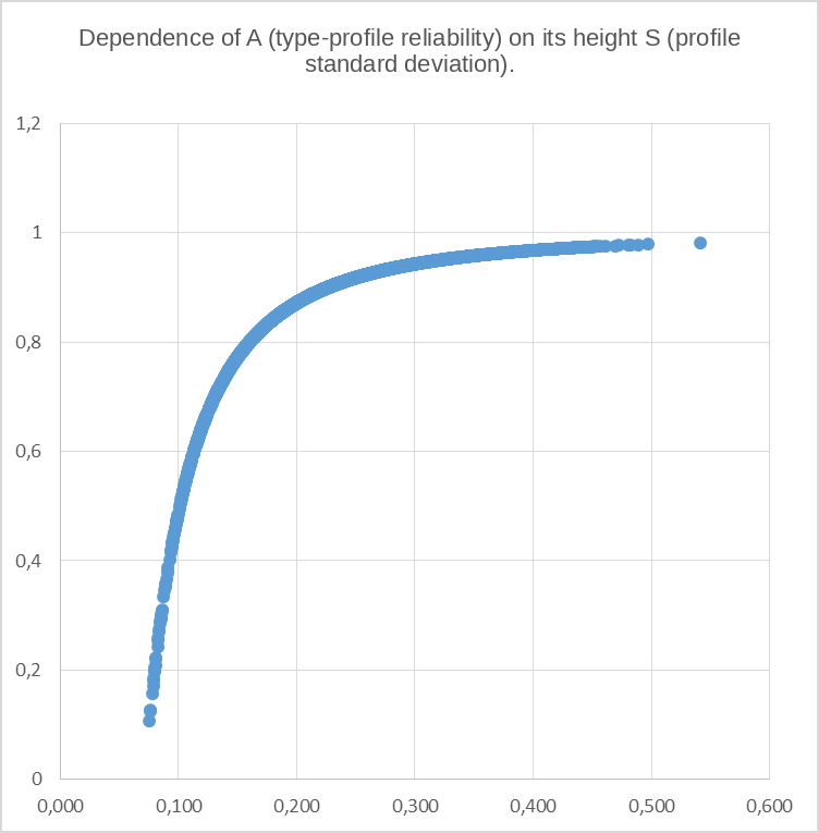
Figure 1
8. Agreement Between the Psychotype from Self-Typing and the Psychotype from Questionnaire Diagnosis as a Function of Respondents’ Individual Test-Reliability Indicators
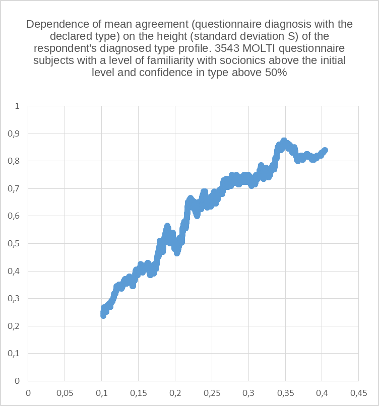
Figure 2. Each point on the graph is averaged over 200 subjects adjacent in the magnitude of S. Sample of 3543 subjects who declared their type with confidence above 50% and whose level of familiarity with socionics was above the initial level.
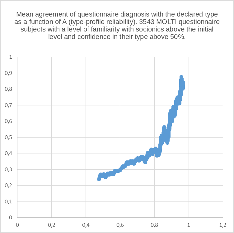
Figure 3. Each point on the graph is averaged over 200 subjects adjacent in the magnitude of A. Sample of 3543 subjects who declared their type with confidence above 50% and whose level of familiarity with socionics was above the initial level.
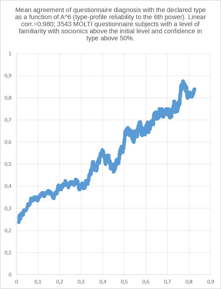
Figure 4. Each point on the graph is averaged over 200 subjects adjacent in the magnitude of A. Sample of 3543 subjects who declared their type with confidence above 50% and whose level of familiarity with socionics was above the initial level.
Let h1, h2, h3 be, respectively, the heights of the 1st (main), 2nd, and 3rd peaks of the diagnosed type profile. From general considerations it is clear that the more strongly the main peak differs in height from the peaks following it in height, that is, the closer the subject is to the center rather than to the boundaries of their type, the greater the agreement between the two diagnoses – questionnaire diagnosis and self-typing – should be. This should occur for two reasons. First, for people who are “non-boundary” cases with respect to their type, their self-typing diagnosis becomes more accurate and reliable. Second, for the same reason, the questionnaire diagnosis also falls “within their own type” more often – in such a case, a large difference in height between the main peak and the secondary peaks is sufficient to preserve the leading position of the “main” peak even when additional stochastic (random) noise, generated by imperfections in questionnaire diagnosis, is superimposed on it and on the secondary peaks. But for the moment this is only a hypothesis requiring verification.
To test it, for each questionnaire profile we construct the function f=(h1+c2*h2+c3*h3)/h1, where c2 and c3 are as yet unknown algebraic numbers (constant coefficients, the weights of the two subsequent profile peaks in the formula). Our task is to find such values of these two coefficients in function f, which characterizes the shape of the profile (and is unrelated to its height), that its correlation with diagnostic agreement, between the questionnaire and self-typing diagnoses, reaches a maximum. This problem is solved using EXCEL software tools (parameter optimization of the solution to maximize the specified criterion). The solution shows that c2 and c3 are indeed negative numbers, and that the maximum correlation of function f with diagnostic agreement (equal to 1 or 0) in a sample of 5790 MOLTI questionnaire respondents with self-declared types is R=0,373, reached at f=(h1-0,425*h2-0,353*h3)/h1
As f increases, the mutual agreement of the questionnaire diagnosis and the self-typing diagnosis increases (Figures 5; 7), and subjects’ confidence in their self-typed type also increases (Figures 6; 8):
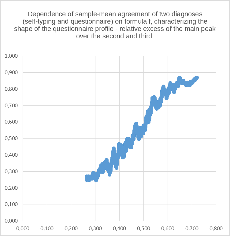
Figure 5. Each point on the graph is averaged over 200 subjects adjacent in the magnitude of f. The graph was constructed using data from all 5790 MOLTI respondents who declared their type (irrespective of their level of familiarity with socionics and percentage confidence in their type).
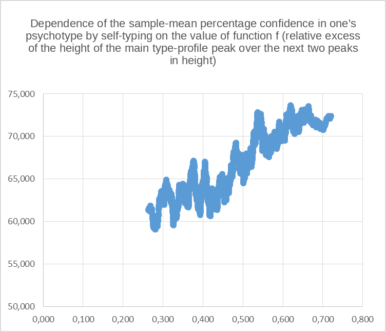
Figure 6. Each point on the graph is averaged over 200 subjects adjacent in the magnitude of f. The graph was constructed using data from all 5790 MOLTI respondents who declared their type (irrespective of their level of familiarity with socionics and percentage confidence in their type).
The graphs show even more contrast in the form of the relationships if only subjects with a level of familiarity with socionics above the initial level are retained when constructing the points (that is, in the coding of the MOLTI questionnaires – with level of familiarity with socionics =2; 3; 4).
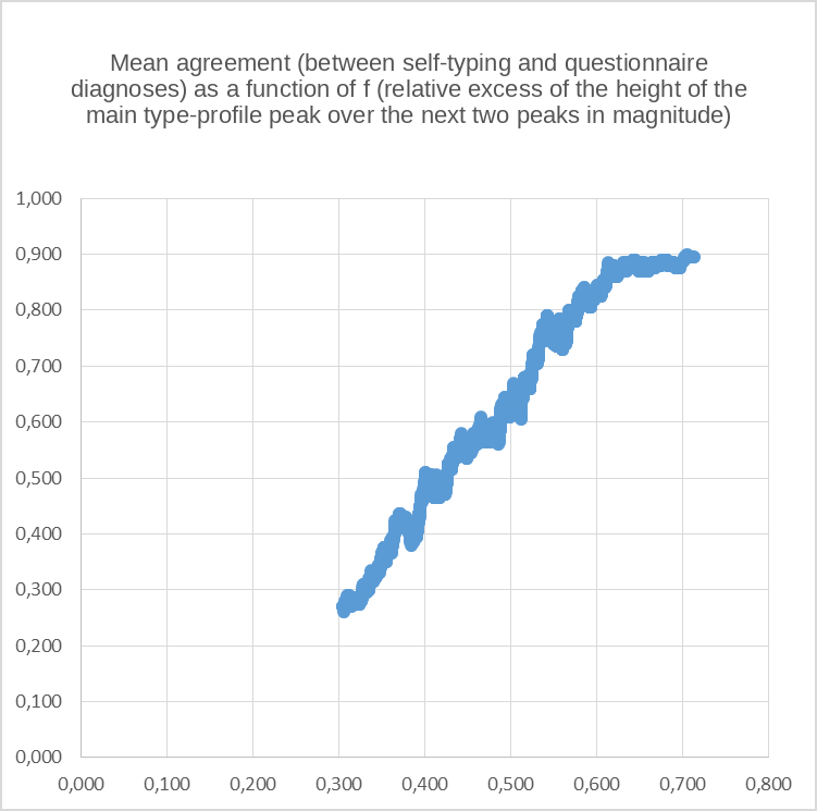
Figure 7. Each point on the graph is averaged over 200 subjects adjacent in the magnitude of f. The graph was constructed using data from 4053 MOLTI respondents who declared their type and indicated a level of familiarity with socionics above the initial level. Initially, as f (the contrast function of the predominance of the main profile peak over the secondary peaks) increases, diagnostic agreement grows linearly, increasing from 0,26 to 0,89, but reaches a plateau (=0,9) beginning at f=0,62.
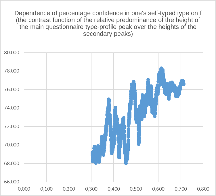
Figure 8. Each point on the graph is averaged over 200 subjects adjacent in the magnitude of f. The graph was constructed using data from 4053 MOLTI respondents who declared their type and indicated a level of familiarity with socionics above the initial level. As f (the contrast function of the predominance of the main profile peak over the secondary peaks) increases, subjects’ mean confidence in their type rises from 69% to 77%.
If the strong influence of f on the agreement between self-typing and questionnaire diagnoses is removed (f being the contrast function of the predominance of the main type-profile peak over the secondary peaks, characterizing the subject’s proximity to the center of the type sector), then the agreement value corrected for this correlation will no longer depend on profile shape, but its dependence on overall profile height (the standard deviation S calculated from the 16 profile values) will remain, and correspondingly so will its dependence on profile reliability A, which is a direct function of S. In this case, as in Figure 4, a linear relationship is again obtained between mean agreement and the sixth power of reliability A (see the following Figure 9):.
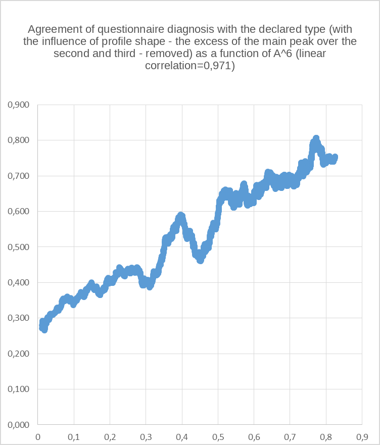
Figure 9. Each point on the graph is averaged over 200 subjects adjacent in the magnitude of A. 3543 MOLTI questionnaire subjects with a level of familiarity with socionics above the initial level and with confidence in their type above 50%. The influence of profile shape, expressed by function f, was preliminarily removed from the agreement measure.
Thus, two independent factors influence the agreement between self-typing and questionnaire diagnoses. The first factor is expressed by function f, which characterizes the shape of the subject’s type profile, namely the relative predominance of the main profile peak over the secondary peaks. The larger function f, the closer the subject is to the center of their type sector and the farther from its boundaries, where the diagnosis (both by self-typing and by questionnaire) becomes unstable. The second factor influencing agreement, which is practically independent of the first, is expressed by the sixth power of type-profile reliability, which in turn is calculated from the standard deviation of the type profile. This second factor characterizes only the individual level of reliability of the subject’s questionnaire answers (and partly also the reliability of their self-typing) and increases in an integrated way as a function of their intelligence, life experience, psychological competence, and motivation (diligence).
These two factors influencing agreement can be summed to obtain a final function explaining the maximum variance in diagnostic agreement (between self-typing and questionnaire diagnosis). Taking into account the different standard deviations of the functions characterizing these two factors (the spread of f is 2,2 times narrower than the spread of A, which should be compensated by multiplying f by 2,2), this optimal factor combination (denote it Z) is: Z= A^6+2,2*f-0,45 = ((S^2-0,0051)/ (S^2))^6+2,2*(h1-0,425*h2-0,353*h3)/h1-0,45 ; where S is the standard deviation of the set of values in each individual type profile obtained from the questionnaire; h1, h2, h3 are the heights of the three largest peaks of this profile in descending order. The weighting coefficient 2,2 before the second factor is determined by differences in each factor’s correlation with agreement and in the magnitude of the standard deviation of the functions expressing them (the first factor is correlated with agreement at 0,322, and the second at 0,373; correspondingly, the sigma of the first factor is 0,217 and that of the second 0,113). The constant term (-0,45) is introduced in order to bring the minimum value of the sum of the factors close to zero.
Across the entire set of MOLTI questionnaire respondents who declared their type by self-typing (5790 people), indicator Z has a linear correlation of 0,460 with the agreement of the two type diagnoses (self-typing and questionnaire diagnosis, with values of 1 or 0). For the correlation of a continuous quantity with a binary-distributed indicator (taking the discrete values 1 or 0), this is a very, very high value of the linear correlation coefficient.
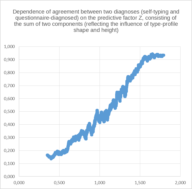
Figure 10. Each point on the graph is averaged over 200 subjects adjacent in the magnitude of Z. The graph was constructed using data from all 5790 MOLTI respondents who declared their type (irrespective of their level of familiarity with socionics and percentage confidence in their type).
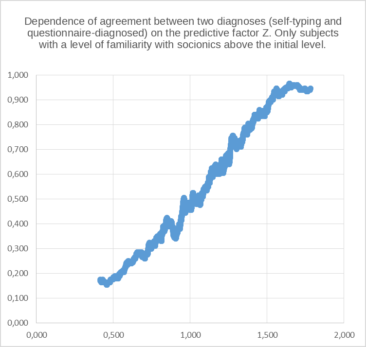
Figure 11. Each point on the graph is averaged over 200 subjects adjacent in the magnitude of Z. The graph was constructed using data from 4053 MOLTI respondents who declared their type and had a level of familiarity with socionics above the initial level.
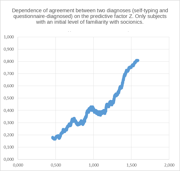
Figure 12. Each point on the graph is averaged over 200 subjects adjacent in the magnitude of Z. The graph was constructed using data from 1737 MOLTI respondents who declared their type and had an initial (minimum) level of familiarity with socionics.
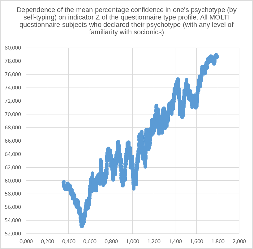
Figure 13. Each point on the graph is averaged over 200 subjects adjacent in the magnitude of Z. The graph was constructed using data from all 5790 MOLTI respondents who declared their type (irrespective of their level of familiarity with socionics and percentage confidence in their type).
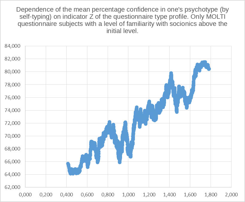
Figure 14. Each point on the graph is averaged over 200 subjects adjacent in the magnitude of Z. The graph was constructed using data from 4053 MOLTI respondents who declared their type and had a level of familiarity with socionics above the initial level.
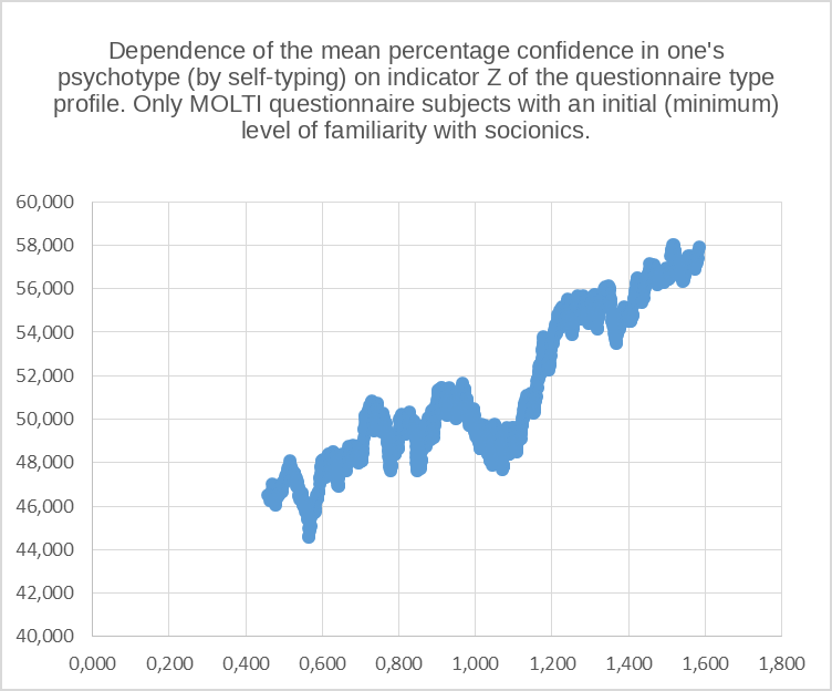
Figure 15. Each point on the graph is averaged over 200 subjects adjacent in the magnitude of Z. The graph was constructed using data from 1737 MOLTI respondents who declared their type and had an initial (minimum) level of familiarity with socionics.
9. Agreement Between the Psychotype from Self-Typing and the Psychotype from Questionnaire Diagnosis as a Function of Respondents’ Sex, Age, and Socionics Experience
Table 10
| Sex | N (number of respondents) | agreement |
|---|---|---|
| 1=male | 2654 | 0,549 |
| 2=female | 7268 | 0,551 |
| Age range | N | agreement |
| 1 | 4694 | 0,531 |
| 2 | 2458 | 0,567 |
| 3 | 1287 | 0,567 |
| 4 | 1001 | 0,566 |
| 5 | 482 | 0,577 |
| Level of familiarity with socionics (from 1 to 4) | N | agreement |
| 1 | 5297 | 0,417 |
| 2 | 3072 | 0,566 |
| 3 | 1316 | 0,697 |
| 4 | 237 | 0,652 |
| probability of TIM by self-assessment (percent) | N | agreement |
| 0 | 192 | 0,427 |
| 5 | 57 | 0,246 |
| 10 | 48 | 0,271 |
| 15 | 42 | 0,310 |
| 20 | 81 | 0,358 |
| 25 | 59 | 0,424 |
| 30 | 156 | 0,333 |
| 35 | 74 | 0,324 |
| 40 | 198 | 0,343 |
| 45 | 88 | 0,341 |
| 50 | 859 | 0,447 |
| 55 | 94 | 0,521 |
| 60 | 354 | 0,506 |
| 65 | 203 | 0,483 |
| 70 | 570 | 0,537 |
| 75 | 340 | 0,597 |
| 80 | 592 | 0,633 |
| 85 | 325 | 0,674 |
| 90 | 513 | 0,704 |
| 95 | 508 | 0,699 |
| 100 | 437 | 0,705 |
Most of the agreement relationships shown in the table are entirely predictable and understandable. Men and women differ little in agreement, but agreement is nevertheless slightly higher among girls/women, which is easily explained by their higher motivation during typing (quite predictably - because women have a greater interest in relationships, creating and strengthening a family, selecting an optimal marriage partner for themselves, etc.). Agreement increases with age, although not very substantially (with age, the life and psychological experience needed for adequate self-assessments accumulates, but intelligent people still remain intelligent and fools remain fools, and this division is no longer related to age and has a much stronger effect on the quality both of self-typing and of questionnaire completion). As the level of familiarity with socionics increases, diagnostic agreement rises quite substantially – however, in what might seem to be the most professional group, the group of socionics “gurus” (237 people), it decreases somewhat again (probably because excessive self-confidence is not always compatible with adequacy). As confidence in one’s declared type increases, agreement indicators likewise increase monotonically in a regular and readily understandable way.
10. Differences in Agreement and Type-Profile Reliability Indicators Depending on the Declared Psychotype – Facts and Analysis of Causes. Main Influencing Factors
Table 11.
| Table of selected indicators of individual type-diagnosis reliability averaged by type groups | 1 | 2 | 3 | 4 | 5 | 6 | 7 | 8 | 9 | 10 | 11 | 12 | 13 | 14 | 15 | 16 | 17 | 18 | 19 | 20 | 21 | 22 | 23 | |
|---|---|---|---|---|---|---|---|---|---|---|---|---|---|---|---|---|---|---|---|---|---|---|---|---|
| ILE | LII | SEI | ESE | SLE | LSI | IEI | EIE | SEE | ESI | ILI | LIE | IEE | EII | SLI | LSE | standard deviation of the indicator in the sample of 5790 people | standard deviation of the indicator in the set of 16 type-group mean values | variance of the indicator in the set of 16 type-group mean values | Association of the indicator with between-type group differences = [18} / [17] | Linear corr. with “blue” A^6 | Linear corr. with “blue” N | Linear corr. with “pink” N | ||
| Calculation of the number of subjects and all mean indicators by type groups identified on the basis of self-typing (5790 respondents with declared types in total) | N (number of respondents with the given TIM) | 359 | 454 | 193 | 139 | 267 | 434 | 743 | 512 | 187 | 316 | 687 | 208 | 420 | 358 | 372 | 141 | 173,8 | 30189,7 | 0,35 | 0,88 | 1,00 | ||
| A | 0,869 | 0,876 | 0,862 | 0,847 | 0,900 | 0,894 | 0,884 | 0,872 | 0,888 | 0,865 | 0,863 | 0,848 | 0,886 | 0,887 | 0,856 | 0,867 | 0,107 | 0,015 | 0,00024 | 0,149 | 0,88 | 0,51 | 0,26 | |
| A^6 | 0,503 | 0,530 | 0,490 | 0,460 | 0,587 | 0,580 | 0,532 | 0,500 | 0,565 | 0,492 | 0,496 | 0,451 | 0,544 | 0,540 | 0,472 | 0,496 | 0,217 | 0,040 | 0,00156 | 0,188 | 0,88 | 0,43 | 0,19 | |
| f | 0,492 | 0,470 | 0,447 | 0,455 | 0,482 | 0,486 | 0,461 | 0,519 | 0,462 | 0,475 | 0,474 | 0,477 | 0,470 | 0,468 | 0,467 | 0,447 | 0,113 | 0,017 | 0,00030 | 0,158 | 0,26 | 0,38 | 0,37 | |
| Z | 1,136 | 1,113 | 1,023 | 1,010 | 1,197 | 1,198 | 1,096 | 1,192 | 1,133 | 1,086 | 1,089 | 1,050 | 1,127 | 1,120 | 1,049 | 1,028 | 0,353 | 0,059 | 0,00348 | 0,172 | 0,76 | 0,53 | 0,37 | |
| agreement of type diagnoses from self-typing and questionnaire | 0,543 | 0,540 | 0,435 | 0,424 | 0,670 | 0,647 | 0,559 | 0,650 | 0,583 | 0,503 | 0,533 | 0,399 | 0,579 | 0,601 | 0,462 | 0,348 | 0,497 | 0,092 | 0,00843 | 0,191 | 0,71 | 0,70 | 0,47 | |
| Calculation of the number of subjects and all mean indicators by type groups identified on the basis of questionnaire typing (5790 respondents with declared types in total) | N (number of respondents with the given TIM) | 301 | 415 | 261 | 180 | 332 | 415 | 639 | 532 | 307 | 310 | 530 | 141 | 446 | 543 | 329 | 109 | 147,2 | 21681,4 | 0,46 | 1,00 | 0,88 | ||
| A | 0,863 | 0,899 | 0,837 | 0,820 | 0,888 | 0,903 | 0,882 | 0,868 | 0,881 | 0,853 | 0,867 | 0,845 | 0,897 | 0,881 | 0,862 | 0,863 | 0,107 | 0,022 | 0,00050 | 0,215 | 0,98 | 0,57 | 0,46 | |
| A^6 | 0,486 | 0,576 | 0,440 | 0,394 | 0,573 | 0,601 | 0,526 | 0,490 | 0,550 | 0,477 | 0,492 | 0,466 | 0,565 | 0,528 | 0,484 | 0,486 | 0,217 | 0,053 | 0,00285 | 0,254 | 1,00 | 0,46 | 0,35 | |
| f | 0,512 | 0,468 | 0,443 | 0,452 | 0,470 | 0,494 | 0,460 | 0,530 | 0,447 | 0,467 | 0,492 | 0,494 | 0,459 | 0,452 | 0,474 | 0,449 | 0,113 | 0,024 | 0,00060 | 0,222 | 0,05 | 0,23 | 0,40 | |
| Z | 1,162 | 1,156 | 0,964 | 0,939 | 1,156 | 1,239 | 1,088 | 1,207 | 1,083 | 1,055 | 1,126 | 1,102 | 1,125 | 1,072 | 1,077 | 1,024 | 0,353 | 0,077 | 0,00601 | 0,226 | 0,72 | 0,48 | 0,52 | |
| agreement of type diagnoses from self-typing and questionnaire | 0,648 | 0,590 | 0,322 | 0,328 | 0,539 | 0,677 | 0,649 | 0,626 | 0,355 | 0,513 | 0,691 | 0,589 | 0,545 | 0,396 | 0,523 | 0,450 | 0,497 | 0,120 | 0,01448 | 0,250 | 0,41 | 0,47 | 0,74 |
According to the results in Table 11, two of its indicators are most strongly associated with between-type differences (see column 20, which reflects this characteristic). These indicators are the agreement of the two diagnoses (questionnaire and self-typing) and the sixth power of indicator A (where A is the individual reliability of the type profile calculated by Cronbach’s method).
Table 12. Full intercorrelation matrix of the indicators from the preceding Table 11, calculated between sets of 16 type-group mean values from the preceding Table 11
| N | A | A^6 | f | Z | agr. | N | A | A^6 | f | Z | agr. | |
|---|---|---|---|---|---|---|---|---|---|---|---|---|
| N | 1,000 | 0,261 | 0,192 | 0,373 | 0,370 | 0,470 | 0,881 | 0,464 | 0,346 | 0,400 | 0,516 | 0,744 |
| A | 0,261 | 1,000 | 0,980 | 0,200 | 0,786 | 0,803 | 0,510 | 0,857 | 0,877 | -0,095 | 0,538 | 0,174 |
| A^6 | 0,192 | 0,980 | 1,000 | 0,154 | 0,769 | 0,786 | 0,429 | 0,839 | 0,883 | -0,127 | 0,520 | 0,134 |
| f | 0,373 | 0,200 | 0,154 | 1,000 | 0,749 | 0,638 | 0,375 | 0,280 | 0,256 | 0,904 | 0,802 | 0,636 |
| Z | 0,370 | 0,786 | 0,769 | 0,749 | 1,000 | 0,939 | 0,530 | 0,743 | 0,757 | 0,499 | 0,867 | 0,501 |
| agreement | 0,470 | 0,803 | 0,786 | 0,638 | 0,939 | 1,000 | 0,704 | 0,709 | 0,709 | 0,343 | 0,725 | 0,380 |
| N | 0,881 | 0,510 | 0,429 | 0,375 | 0,530 | 0,704 | 1,000 | 0,569 | 0,463 | 0,226 | 0,475 | 0,469 |
| A | 0,464 | 0,857 | 0,839 | 0,280 | 0,743 | 0,709 | 0,569 | 1,000 | 0,980 | 0,089 | 0,736 | 0,465 |
| A^6 | 0,346 | 0,877 | 0,883 | 0,256 | 0,757 | 0,709 | 0,463 | 0,980 | 1,000 | 0,048 | 0,722 | 0,408 |
| f | 0,400 | -0,095 | -0,127 | 0,904 | 0,499 | 0,343 | 0,226 | 0,089 | 0,048 | 1,000 | 0,726 | 0,753 |
| Z | 0,516 | 0,538 | 0,520 | 0,802 | 0,867 | 0,725 | 0,475 | 0,736 | 0,722 | 0,726 | 1,000 | 0,802 |
| agreement | 0,744 | 0,174 | 0,134 | 0,636 | 0,501 | 0,380 | 0,469 | 0,465 | 0,408 | 0,753 | 0,802 | 1,000 |
As we can see, almost all indicators prove to be sufficiently stable with respect to the method used to identify the type groups (self-typing or questionnaire). The sole exception is agreement, for which the correlation between the two type series identified by the two different methods is fairly moderate (+0,380).
An important fact in the tables is that all type-group mean reliability indicators without exception (and validity indicators as well, when agreement is concerned) are substantially positively correlated with the size N of the corresponding type groups in the sample. The correlations between type-group size and the mean agreement of the two diagnoses within those groups (questionnaire and self-typing) are especially strong. We shall analyze the reasons for this in detail below.
Diagnostic agreement (questionnaire and self-typing) turned out to differ substantially among the different type groups. This is not a random result. Differences in mean diagnostic agreement (between self-typing and the results of diagnostic questionnaires) in different respondent type groups arise under the influence of three main causes: 1) dependence of the consistency of psychological self-assessments on the subjects’ type (the factor of type-dependent competence in psychological self-assessment); 2) the factor of the social “fashionability” (or unfashionability) of each psychotype; 3) the size of the type groups (that is, type frequency in the sample). Groups of rare types are more contaminated by extraneous errors than groups of frequent types. We shall call this effect (an explanation of it will be provided below) the error-diffusion effect.
We shall now examine all factors influencing agreement in greater detail:
11. First Factor - Different Competence in Psychological Self-Assessment Among Representatives of Different Psychotypes When Reflecting and Understanding Their Own Psychological Properties in Comparison with Other People
We shall call this factor the “psychological self-assessment competence factor.” This factor affects the consistency of a person’s psychological self-assessments and manifests itself directly and primarily in the height of the type profile obtained for that person from the questionnaire, as well as in quantities related to this height (see indicators A and A^6 in the table). The factor’s influence is also transmitted indirectly to agreement, because the magnitude of agreement likewise depends on A^6. The factor is, of course, an individual characteristic of a person, but it also exhibits substantial between-TIM differences. The magnitude of the “blue” A^6 in the table (that is, the mean values of this indicator in each of the 16 type groups assembled on the basis of questionnaire diagnosis) most directly and accurately reflects the mean magnitude of this factor for each TIM. For psychotypes in which this factor is higher, it slightly increases the size of the corresponding type groups (both when they are formed from questionnaire-diagnosis results and when they are formed from self-typing results) – because more accurate diagnosis reduces the outflow of true representatives of the corresponding TIM from the type group corresponding to it, formed by the results of either type of diagnosis (questionnaire or self-typing). It should be noted in particular that psychological competence in self-assessment is unlikely to be closely positively associated with psychological competence in assessing other people. In the present study, we do not examine the subject’s assessments of other people (although precisely this kind of psychological competence would be useful to socionic typers and type diagnosticians).
12. Second Factor - Fashionable and Unfashionable Types
This second factor consists in the effect of a psychotype’s degree of “social fashionability.” The degree of fashionability (and hence of social preference) depends mainly on the socionic stereotypes (positive or negative) that form in the mass consciousness of people who are familiar with socionics or are beginning to become familiar with it, on the basis of the various psychotype descriptions posted on the Internet. The factor of the social fashionability of psychotypes does not affect the individual reliability of the resulting type profile (that is, indicators A and A^6); it affects only mean group agreement in type groups identified from self-typing results – reducing it for “fashionable” types because, through its influence, some of the psychotypes in these groups are identified incorrectly (outsiders like to classify themselves as fashionable types). This factor leads to actual diagnostic errors only in self-typing; in questionnaire diagnosis it does not lead to diagnostic errors. But it nevertheless indirectly affects agreement within type groups formed from questionnaire-diagnosis results as well (because agreement is the proportion of matches between two diagnoses, one of which is the self-typing diagnosis).
“Fashionable” psychotypes attract erroneous self-typings from representatives of nearby, adjacent types. For this reason, the agreement indicator in groups of “fashionable” types decreases if those types are defined by self-typing results, while the size of those groups increases (because of its “fashionability,” the type becomes excessively diluted by representatives of other types, that is, it contains a higher percentage of “false alarms”). In short, if the type group of some “fashionable” type is formed on the basis of self-typing, the percentage of errors in it will be higher (because many representatives of “non-own” types are attracted to the fashionable type during self-typing diagnosis). Conversely, if the type group of representatives of this same “fashionable type” is formed on the basis of questionnaire diagnoses, the mean reliability of questionnaire diagnoses in this group does not change, whereas the group mean reliability of self-typing diagnoses actually increases rather than decreases (the percentage of errors decreases) – because in this case outside types are no longer attracted into the group by definition, while “own types” are not lost from it as a result of self-typing (true representatives of the “fashionable type” less often leave for an “alien” type as a result of self-typing, because they have no socially “fashionable” need to do so). Thus, when type groups are formed by questionnaire diagnosis, the factor’s influence on agreement in the type group of a “fashionable type” becomes positive rather than negative. Let us formulate once again, and somewhat differently, why this occurs. If a group of some “fashionable” type is formed from purely questionnaire-based diagnosis, there will be no outsiders excessively attracted to that group because of the type’s “fashionability,” whereas a higher proportion of true representatives of that type will receive their true diagnosis through self-typing (because true representatives of a “fashionable type,” during self-typing into a “fashionable type,” have no need deliberately to “run away” from their true type diagnosis).
As a result of these two oppositely directed mechanisms, across the series of 16 types this factor should be negatively correlated with their mean type-group agreement when the type groups are formed from self-typing results, and should be positively correlated with mean type-group agreement when the type groups are formed from questionnaire-diagnosis results. The factor has a positive effect on the size of type groups of “fashionable types” formed from self-typing results (artificially increasing their size), and has no effect at all on the size of groups formed from questionnaire-diagnosis results. The factor likewise has no effect on individual indicators of type-profile reliability (its height S and the reliability indicators A and A^6 associated with it), or on the group mean values of these indicators.
To quantitatively estimate the social fashionability-unfashionability of a psychotype, it is sufficient to calculate the ratio of the size of the corresponding type group according to self-typing data to the size of the same type group in the sample according to questionnaire-diagnosis data (because in the latter case the sizes of the type groups are free from the influence of the type-fashionability factor). It is true that, before doing this, it is better to remove from the sizes of the corresponding type groups the influence of the preceding factor - the factor of different competence in psychological self-assessment among representatives of different types. In those type groups in which this psychological competence is higher, the psychological-competence factor increases the size of the corresponding groups (because it reduces the outflow from these groups of true representatives of the type). This influence on group size must be removed beforehand if we need to calculate, for each psychotype (from the ratio of the sizes of the corresponding type groups), the magnitude of the second factor, the factor of the type’s social fashionability.
The results of these operations are presented in the following Table 13:
Table 13
| ILE | LII | SEI | ESE | SLE | LSI | IEI | EIE | SEE | ESI | ILI | LIE | IEE | EII | SLI | LSE | ||||||
|---|---|---|---|---|---|---|---|---|---|---|---|---|---|---|---|---|---|---|---|---|---|
| 1 | before correction to remove correlation with A^6 | self-typing | N (number of respondents with the given TIM) | 359 | 454 | 193 | 139 | 267 | 434 | 743 | 512 | 187 | 316 | 687 | 208 | 420 | 358 | 372 | 141 | ||
| 2 | before correction to remove correlation with A^6 | questionnaire diagnosis | N (number of respondents with the given TIM) | 301 | 415 | 261 | 180 | 332 | 415 | 639 | 532 | 307 | 310 | 530 | 141 | 446 | 543 | 329 | 109 | ||
| 3 | before correction to remove correlation with A^6 | questionnaire diagnosis | A^6 | 0,486 | 0,576 | 0,440 | 0,394 | 0,573 | 0,601 | 0,526 | 0,490 | 0,550 | 0,477 | 0,492 | 0,466 | 0,565 | 0,528 | 0,484 | 0,486 | ||
| 4 | Psychological self-assessment competence factor depending on TIM (values in row 3 normalized to a zero mean and unit standard deviation) | -0,42 | 1,26 | -1,28 | -2,15 | 1,20 | 1,74 | 0,33 | -0,34 | 0,77 | -0,58 | -0,30 | -0,80 | 1,06 | 0,36 | -0,45 | -0,41 | ||||
| 5 | after correction to remove correlation with the psychological-competence factor (row 4) | self-typing | N (number of respondents with the given TIM) | 384,4 | 377,3 | 270,9 | 269,6 | 193,8 | 328,2 | 722,8 | 532,5 | 140,1 | 351,3 | 705,3 | 256,7 | 355,8 | 336 | 399,3 | 166,1 | ||
| 6 | after correction to remove correlation with the psychological-competence factor (row 4) | questionnaire diagnosis | N (number of respondents with the given TIM) | 329,2 | 329,5 | 347,8 | 325,5 | 250,5 | 297,1 | 616,5 | 554,8 | 254,7 | 349,3 | 550,4 | 195,2 | 374,5 | 518,5 | 359,4 | 136,9 | ||
| 7 | Final indicator of the psychotype’s “social fashionability” (element in row 5 divided by the element in row 6) | 1,17 | 1,14 | 0,78 | 0,83 | 0,77 | 1,10 | 1,17 | 0,96 | 0,55 | 1,01 | 1,28 | 1,31 | 0,95 | 0,65 | 1,11 | 1,21 | ||||
| 8 | Normalized magnitude of the “social fashionability” factor (row 7 brought to a zero mean and unit standard deviation) | 0,75 | 0,65 | -1,00 | -0,78 | -1,02 | 0,47 | 0,78 | -0,18 | -2,03 | 0,02 | 1,27 | 1,42 | -0,23 | -1,59 | 0,50 | 0,96 | ||||
| 9 | after final correction to remove correlation also with the social-fashionability factor (row 8) | self-typing | N (number of respondents with the given TIM) | 327,4 | 328,0 | 346,2 | 328,1 | 270,9 | 292,7 | 664,2 | 546,2 | 293,4 | 349,4 | 609,6 | 149,6 | 372,9 | 455,9 | 361,6 | 93,7 |
The table shows that the psychological self-assessment competence factor (row 4 of the table) is highest (in descending order) among representatives of the LSI, LII, SLE, IEE, and SEE types. Its lowest values are found among the Alpha ethical types ESE and SEI.
The “social fashionability” factor of psychotypes is highest among “black” logicians and intuitives. In descending order, elevated popularity is found for: LIE, ILI, LSE, IEI, ILE, LII. The greatest negative popularity is found for SEE, EII, SLE, SEI, ESE.
The last row of the table presents the sizes of type groups formed from self-typing results after corrections have been introduced for both factors: psychological competence and social fashionability. Before any corrections for these factors were introduced, the sizes of the type groups formed from self-typing and questionnaire-diagnosis results correlated with one another across the series of 16 psychotypes at a level of 0,88. After correction for the factor of mean psychological competence of different TIMs was introduced, the correlation remained at a level of 0,87. But after the final correction for the social-fashionability factor was introduced into the sizes of the type groups formed from self-typing results, the correlation between the two series of type-group sizes increased to 0,98.
Below we present another table, Table 14 – containing linear correlations that various indicators of mean reliability and mean agreement in type groups exhibit, across series of 16 type-group mean values, first with the finally corrected sizes of the corresponding type groups and, second, with the two factors considered above: the psychological self-assessment competence factor and the social fashionability factor of TIMs.
Table 14.
| correlation with TIM frequency in the MOLTI questionnaire corrected for the competence factor | correlation with TIM frequency from self-typing results corrected for the competence and fashionability factors | correlation with the psychological self-assessment competence factor | correlation with the TIM fashionability factor | ||
|---|---|---|---|---|---|
| Series of 16 type-group mean values of the indicator, with type groups formed from the MOLTI questionnaire. Without corrections. | N (number of respondents with the given TIM according to questionnaire diagnosis - MOLTI) | 0,89 | 0,88 | 0,46 | -0,04 |
| Series of 16 type-group mean values of the indicator, with type groups formed from the MOLTI questionnaire. Without corrections. | A | 0,14 | 0,16 | 0,98 | -0,01 |
| Series of 16 type-group mean values of the indicator, with type groups formed from the MOLTI questionnaire. Without corrections. | A^6 (normalized values of this indicator form the psychological self-assessment competence factor) | 0,00 | 0,03 | 1,00 | -0,08 |
| Series of 16 type-group mean values of the indicator, with type groups formed from the MOLTI questionnaire. Without corrections. | f | 0,23 | 0,21 | 0,05 | 0,48 |
| Series of 16 type-group mean values of the indicator, with type groups formed from the MOLTI questionnaire. Without corrections. | agreement of type diagnoses from self-typing and questionnaire | 0,32 | 0,34 | 0,41 | 0,73 |
| Series of 16 type-group mean values of the indicator, with type groups formed from self-typing results. Without corrections. | N (number of respondents with the given TIM according to self-typing results) | 0,81 | 0,84 | 0,35 | 0,41 |
| Series of 16 type-group mean values of the indicator, with type groups formed from self-typing results. Without corrections. | A | 0,12 | 0,15 | 0,88 | -0,39 |
| Series of 16 type-group mean values of the indicator, with type groups formed from self-typing results. Without corrections. | A^6 | 0,03 | 0,08 | 0,88 | -0,41 |
| Series of 16 type-group mean values of the indicator, with type groups formed from self-typing results. Without corrections. | f | 0,28 | 0,26 | 0,25 | 0,15 |
| Series of 16 type-group mean values of the indicator, with type groups formed from self-typing results. Without corrections. | agreement of type diagnoses from self-typing and questionnaire | 0,43 | 0,45 | 0,71 | -0,35 |
| Series of 16 type-group mean values of the indicator, with type groups formed from the MOLTI questionnaire. After correction for the psychological-competence factor. | N - TIM frequency after correction for the psychological-competence factor | 1,00 | 0,98 | 0,00 | 0,00 |
| Series of 16 type-group mean values of the indicator, with type groups formed from self-typing results. After correction for the psychological-competence and social-fashionability factors | N - TIM frequency after correction for the psychological-competence and social-fashionability factors | 0,98 | 1,00 | 0,03 | 0,00 |
| TIM fashionability factor | 0,00 | 0,00 | -0,07 | 1,00 |
Correlations especially important to the present discussion are highlighted in yellow in the table. First, we see (as predicted above) that the TIM fashionability factor correlates positively (+0,73) with agreement across different TIM groups when they were identified on the basis of questionnaire diagnoses, and correlates negatively (-0,35) with analogous agreement across different TIM groups when the groups were formed on the basis of self-typing. Second, the correlation of mean type-group agreement with TIM frequency (that is, with the sizes of the corresponding type groups) is greater when the groups are formed from self-typing results (+0,45) than when they are formed from questionnaire-diagnosis results (+0,32). This result is related to the fact that the probability of correctly identifying type is lower in self-typing than in questionnaire diagnosis, and consequently the error-diffusion effect that produces this correlation, and which will be discussed in greater detail in the next paragraph, is larger in the case of self-typing.
13. Third Factor - Diffusion of Errors from Frequent Types to Rare Types
The essence of this effect lies in the mutual diffusion of false-recognition errors (false alarms) from types adjacent in their properties. This effect is not symmetrical for types that are objectively rarer and more frequent in the subpopulation being examined. It manifests much more strongly for psychotypes that occur rarely in the subpopulation. Specifically, within type groups of objectively rare types, mean agreement indicators decrease because these type groups are internally diluted by erroneous assignments of people to the type much more often (in a larger percentage of cases) than occurs for types that are objectively frequent in the subpopulation. Why is this so? Let us explain using the example of a hypothetical subpopulation under examination that, for simplicity, consists only of representatives of two types: LIE and LII. Let there be objectively four times as many LII representatives as LIE representatives in the population (400 LII + 100 LIE). Thus, LII is a frequent type for this subpopulation, and LIE is a rare type. If we know that the sample consists only of these two types and subsequent type diagnosis in this sample is performed with 100% reliability, then all types are identified absolutely accurately and no errors arise for either type. If diagnosis is performed with 90% reliability, then 90% of all LII (360 people) and 90% of all LIE (90 people) will be correctly assigned to their own type, but 10% of LII (40 people) will be erroneously assigned to LIE, just as 10% of true LIE (10 people) will be erroneously assigned to LII. As a result, in the group diagnosed as LII we will have a total of 370 people (fewer than the true 400), of whom 360 will be genuine LII (97,3%) and 10 people (2,7%) representatives of an “alien” type. In the LIE group, which was rarer to begin with, diagnosis will produce 130 people (more than there should be), of whom only 90 (69,2%) are genuine LIE and 40 (30,8%) are representatives of the “alien” type. The asymmetry of the situation becomes even more pronounced if diagnostic reliability decreases further. Let it now be 70%. In this case, 280 LII and 70 LIE will be correctly assigned to their own type, 120 people will be erroneously assigned to LIE, and 30 people will be erroneously assigned to LII. In total, we will have 310 diagnosed LII, of whom 280 (90,3%) will be correctly diagnosed and 30 (9,7%) incorrectly diagnosed. The situation will be much worse for the initially rare LIE type. A total of 190 people will be diagnosed as LIE, of whom only 70 will be correct (36,8%) and a much larger number, 120 people (63,2%), will be incorrect.
This is the effect of asymmetric error diffusion. It leads to the appearance of stable positive correlations between mean agreement within each type group identified by the results of less-than-perfect diagnosis and the size of that type group. For objectively frequent types, the error-diffusion factor slightly reduces their diagnosed frequency and has little effect on the reliability with which they are identified, but for objectively rare types it artificially (and substantially in percentage terms) inflates the size of the corresponding type group and sharply reduces diagnostic-reliability indicators within that group because it strongly dilutes the group with representatives of “alien” types. The error-diffusion effect occurs both in self-typing and in questionnaire diagnosis. But it is always more strongly expressed in cases in which diagnostic reliability was lower to begin with. For example, if the reliability of self-typing is lower than the reliability of questionnaire diagnosis, the error-diffusion effect will be stronger for self-typing, and in particular, for groups of “rare” types (and only for them) formed from self-typing results, mean diagnostic-agreement indicators within these groups will be reliably and much lower than within the same-named type groups formed from the results of the more reliable diagnostic procedure.
Unfortunately, a reverse correction, that is, direct correction of the empirically identified sizes of type groups on the basis of their positive correlation with mean agreement within those groups, cannot be performed (in this case, the positive correlation of the empirically identified TIM frequency with agreement within type groups indicates not an overestimation but precisely an underestimation of the frequency of frequent TIMs and an overestimation of the frequency of rare ones – therefore, an attempt to correct group sizes by eliminating the correlation with agreement would only produce the opposite result, increasing still further the error in determining the true frequencies of the types). In fact, it is entirely possible to construct a mathematical model for the real correction of type frequencies - ultimately yielding the frequency of the actual representation of true TIMs in the subpopulation. But we will not do this in the present article, so as not to burden it with additional derivations. For the present purpose, it is sufficient to use refined type frequencies corrected for the parasitic influence of two factors (psychological competence and social fashionability) and then to take a weighted average of the independent self-typing and questionnaire-diagnosis data with weights of 0,63 and 0,83, respectively (these weights are obtained in the subsequent section of the article, “Calculation and comparison of the mean probability of identifying the true type in self-typing and in MOLTI questionnaire diagnosis”; they reflect the mean reliability of type diagnosis by self-typing and by the MOLTI questionnaire). The final frequencies of psychotypes in the Internet sample of MOLTI respondents, from which the parasitic noise-producing influence of differences in psychological competence and differences in the social fashionability of TIMs has been removed, together with the normalized values of the error-diffusion factor obtained from these corrected frequency indicators, are presented in the following Table 15:
Table 15.
| ILE | LII | SEI | ESE | SLE | LSI | IEI | EIE | SEE | ESI | ILI | LIE | IEE | EII | SLI | LSE | |
|---|---|---|---|---|---|---|---|---|---|---|---|---|---|---|---|---|
| Absolute number of TIMs in the sample (with correction for the factors of psychological competence and social fashionability of TIMs) | 328,4 | 328,9 | 347,1 | 326,6 | 259,3 | 295,2 | 637,1 | 551,1 | 271,4 | 349,3 | 575,9 | 175,5 | 373,8 | 491,5 | 360,3 | 118,3 |
| Corresponding number of TIMs as proportions of the sample | 0,057 | 0,057 | 0,060 | 0,056 | 0,045 | 0,051 | 0,110 | 0,095 | 0,047 | 0,060 | 0,099 | 0,030 | 0,065 | 0,085 | 0,062 | 0,020 |
| Values of frequency normalized (to a zero mean and unit standard deviation) - normalized values of the error-diffusion factor | -0,25 | -0,24 | -0,11 | -0,26 | -0,75 | -0,49 | 2,03 | 1,39 | -0,67 | -0,09 | 1,58 | -1,37 | 0,09 | 0,95 | -0,01 | -1,79 |
As we can see, the rarest type in the Internet sample is LSE (no more than 2%), and the most frequent is its conflictor IEI (at least 11%)..
14. Fourth and Final Factor Affecting Between-Type Differences in Mean Diagnostic Agreement – the Factor of Mean Distance from the TIM’s Location in Multidimensional Psychological Space to the Locations of Other TIMs (Factor of the TIM’s Mean Remoteness from the Other 15 TIMs)
The influence of error diffusion on group mean agreement indicators can be eliminated by correcting all type-group mean agreement indicators for their correlation with the resulting size of the corresponding type groups. The correlation of type-group mean agreement values with the factors of different psychological competence and TIM fashionability can also be removed. For the corrected agreement values (from which the influences of all three factors - competence, fashionability, and error diffusion - have been completely removed), we then obtain the following Table 16, where these agreement values occupy its first two columns, while the remaining columns contain values of function f averaged by type group (both without correction for the three factors already known to us to influence agreement and with correction for them). It turns out that the values of function f averaged by type group and corrected for their small correlations with the three preceding factors constitute the final sought fourth factor influencing agreement. There can no longer be a fifth factor, because after the fourth factor the variance of differences in agreement among the 16 type groups is practically exhausted.
Recall also that function f (which precisely reflects the factor of the TIM’s mean remoteness from the other 15 TIMs) was introduced in Section 8 of the article.
Table 16.
| 1 | 2 | 3 | 4 | 5 | 6 | 7 | 8 | |
|---|---|---|---|---|---|---|---|---|
| Agreement of type diagnoses (self-typing and questionnaire). Type-group mean values in type groups identified on the basis of questionnaire diagnoses. Values are corrected for the competence, fashionability, and error-diffusion factors. | Agreement of type diagnoses (self-typing and questionnaire). Type-group mean values in type groups identified on the basis of self-typing. Values are corrected for the competence, fashionability, and error-diffusion factors. | Function f averaged over type groups identified on the basis of the questionnaire (function f is described in the sections above and characterizes the degree to which the main profile peak exceeds the second- and third-highest peaks). The greater f is, the more accurate the diagnosis - the less competition the main peak, the candidate for TIM, receives from the secondary peaks. Recall that f=(h1-0,425*h2-0,353*h3)/h1, where h1, h2, h3 are, respectively, the heights of the 1st (main), 2nd, and 3rd peaks of the diagnosed type profile. | Function f averaged over type groups identified on the basis of self-typing (function f is described in the sections above and characterizes the degree to which the main profile peak exceeds the second- and third-highest peaks). The greater f is, the more accurate the diagnosis - the less competition the main peak, the candidate for TIM, receives from the secondary peaks. Recall that f=(h1-0,425*h2-0,353*h3)/h1, where h1, h2, h3 are, respectively, the heights of the 1st (main), 2nd, and 3rd peaks of the diagnosed type profile. | Function f averaged over type groups identified on the basis of the questionnaire - with correction (with the influence of three factors - competence, fashionability, and error diffusion - removed) | Function f averaged over type groups identified on the basis of self-typing - with correction (with the influence of three factors - competence, fashionability, and error diffusion - removed) | Function f averaged across the two methods of identifying type groups. (Averaging of the indicators in columns 5 and 6) | Sought Factor No. 4 - normalized values of column 7. | |
| ILE | 0,612 | 0,604 | 0,512 | 0,492 | 0,505 | 0,493 | 0,499 | 1,480 |
| LII | 0,481 | 0,488 | 0,468 | 0,470 | 0,460 | 0,464 | 0,462 | -0,561 |
| SEI | 0,476 | 0,490 | 0,443 | 0,447 | 0,457 | 0,456 | 0,456 | -0,896 |
| ESE | 0,512 | 0,548 | 0,452 | 0,455 | 0,465 | 0,467 | 0,466 | -0,338 |
| SLE | 0,602 | 0,583 | 0,470 | 0,482 | 0,485 | 0,483 | 0,484 | 0,637 |
| LSI | 0,570 | 0,568 | 0,494 | 0,486 | 0,489 | 0,480 | 0,484 | 0,670 |
| IEI | 0,490 | 0,481 | 0,460 | 0,461 | 0,440 | 0,447 | 0,444 | -1,594 |
| EIE | 0,602 | 0,617 | 0,530 | 0,519 | 0,524 | 0,515 | 0,519 | 2,608 |
| SEE | 0,526 | 0,486 | 0,447 | 0,462 | 0,474 | 0,466 | 0,470 | -0,117 |
| ESI | 0,543 | 0,545 | 0,467 | 0,475 | 0,468 | 0,478 | 0,473 | 0,032 |
| ILI | 0,539 | 0,527 | 0,492 | 0,474 | 0,470 | 0,464 | 0,467 | -0,317 |
| LIE | 0,553 | 0,554 | 0,494 | 0,477 | 0,486 | 0,484 | 0,485 | 0,686 |
| IEE | 0,510 | 0,500 | 0,459 | 0,470 | 0,460 | 0,466 | 0,463 | -0,529 |
| EII | 0,472 | 0,501 | 0,452 | 0,468 | 0,463 | 0,467 | 0,465 | -0,386 |
| SLI | 0,502 | 0,507 | 0,474 | 0,467 | 0,469 | 0,468 | 0,468 | -0,227 |
| LSE | 0,452 | 0,478 | 0,449 | 0,447 | 0,448 | 0,455 | 0,452 | -1,147 |
| correlation of column 1 with the others | 1 | 0,922 | 0,781 | 0,831 | 0,874 | 0,840 | 0,867 | 0,867 |
| correlation of column 2 with the others | 0,922 | 1 | 0,810 | 0,834 | 0,897 | 0,908 | 0,910 | 0,910 |
In conclusion to the analysis of all four factors influencing differences among the 16 type-group mean agreement indicators, we present Tables 17 and 18 with characteristics and with the complete socionic decomposition (by types, traits, and functions) for all four normalized factors influencing agreement:
Table 17.
| factor of psychological self-assessment competence linked to TIM | factor of the type’s social fashionability | error-diffusion factor (linked not to TIM but to its proportion in the sample - in this case calculated for the Internet sample of MOLTI questionnaire respondents) | Factor by which the first harmonic exceeds the second and third in the mean type profile of TIM representatives. Objectively linked to TIM, to its location in psychological space, and to its distance in that space from the nearest neighboring TIMs (potential competitors in diagnosis) | |
|---|---|---|---|---|
| Comments on the factor | Errors inevitable in diagnosis, in which a person is assigned not to their own TIM but to an alien TIM, are distributed unevenly in the sample - their relative proportion is higher in groups of types rare in the sample and lower in groups of frequent types. This is the essence of the factor. It is linked not to TIM itself, but to its proportion in the sample, that is, to the situational frequency of the TIM in a particular sample. For samples with different TIM frequency compositions, the factor values associated with the TIMs also differ. | The factor is measured as the normalized value of f, first averaged over the type group of subjects, from which the influence of the three preceding factors has been removed (which changes it only very slightly, because the correlations of f with these factors are minimal). Recall that f=(h1-0,425*h2-0,353*h3)/h1, where h1, h2, h3 are, respectively, the heights of the 1st (main), 2nd, and 3rd peaks of the diagnosed type profile. The greater f is, the greater the mean distance in the type group of subjects between the highest profile peak and the next two peaks in height, and therefore the less frequently diagnostic errors occur. In terms of another metaphor, the location of a TIM in multidimensional psychological space, a high factor value corresponds to TIMs that are far from neighboring TIMs in that space and occupy the most isolated position. | ||
| Effects of the factor in type groups formed from self-typing results | The factor increases the accuracy of self-typing diagnosis. High factor values increase mean type-group agreement and, more moderately, increase the size of this type group (preventing the outflow of true representatives of the TIM from it) | The factor affects the results of self-typing diagnosis. High factor values reduce mean type-group agreement (because of the inflow of spurious representatives into the type group) and increase the size of this type group (because of the inflow of spurious representatives into it) | High factor values contribute to increased mean type-group agreement (because of increased outflow from the type group of cases with erroneous diagnoses into other type groups in which the value of this factor is below average - mean agreement there falls as a result) | High factor values correspond to low competing interference from other TIMs during diagnosis (the TIM is remote in its properties from all other neighbors). Therefore, high factor values reduce the probability of diagnostic errors and thereby increase agreement. |
| Effects of the factor in type groups formed from MOLTI questionnaire-diagnosis results | The factor increases the accuracy of questionnaire diagnosis. High factor values increase mean type-group agreement and increase the size of this type group (preventing the outflow of true representatives of the TIM from it) | High factor values substantially increase mean type-group agreement (exclusively because true representatives of the TIM, according to their self-typing results as well, almost all receive, without losses in frequency, the correct “fashionable” diagnosis, which in this case coincides with the questionnaire diagnosis). The factor has no effect on the size of the type group identified from the questionnaire diagnosis (because it has no effect on the questionnaire diagnosis itself). | High factor values contribute to increased mean type-group agreement (because of increased outflow from the type group of cases with erroneous diagnoses into other type groups in which the value of this factor is below average - mean agreement there falls as a result) | High factor values correspond to low competing interference from other TIMs during diagnosis (the TIM is remote in its properties from all other neighbors). Therefore, high factor values reduce the probability of diagnostic errors and thereby increase agreement. |
| proportion of variance in the spread of the agreement indicator across the 16 type groups formed from self-typing results that is associated with the factor (in parentheses - the correlation of agreement with factor values in type groups formed by self-typing) | 0,495 (0,708) | 0,122 (—0,351) | 0,191 (0,439) | 0,188 (0,437) |
| proportion of variance in the spread of the agreement indicator across the 16 type groups formed from MOLTI questionnaire-diagnosis results that is associated with the factor (in parentheses - the correlation of agreement with factor values in type groups formed by questionnaire diagnosis) | 0,166 (0,408) | 0,529 (0,727) | 0,109 (0,330) | 0,135 (0,367) |
Table 18. Weight loadings of the four factors influencing type-group mean agreement indicators, projected onto types, functions, and trait poles:
| factor of psychological self-assessment competence linked to TIM | factor of the type’s social fashionability | error-diffusion factor (linked not to TIM but to its proportion in the sample - in this case calculated for the Internet sample of MOLTI questionnaire respondents) | Factor by which the first harmonic exceeds the second and third in the mean type profile of TIM representatives. Objectively linked to TIM, to its location in psychological space, and to its distance in that space from the nearest neighboring TIMs (potential competitors in diagnosis) | |
|---|---|---|---|---|
| ILE | -0,42 | 0,75 | -0,25 | 1,48 |
| LII | 1,26 | 0,65 | -0,24 | -0,56 |
| SEI | -1,28 | -1,00 | -0,11 | -0,90 |
| ESE | -2,15 | -0,78 | -0,26 | -0,34 |
| SLE | 1,20 | -1,02 | -0,75 | 0,64 |
| LSI | 1,74 | 0,47 | -0,49 | 0,67 |
| IEI | 0,33 | 0,78 | 2,03 | -1,59 |
| EIE | -0,34 | -0,18 | 1,39 | 2,61 |
| SEE | 0,77 | -2,03 | -0,67 | -0,12 |
| ESI | -0,58 | 0,02 | -0,09 | 0,03 |
| ILI | -0,30 | 1,27 | 1,58 | -0,32 |
| LIE | -0,80 | 1,42 | -1,37 | 0,69 |
| IEE | 1,06 | -0,23 | 0,09 | -0,53 |
| EII | 0,36 | -1,59 | 0,95 | -0,39 |
| SLI | -0,45 | 0,50 | -0,01 | -0,23 |
| LSE | -0,41 | 0,96 | -1,79 | -1,15 |
| EXTRAVERT | -0,136 | -0,138 | -0,451 | 0,410 |
| IRRATIONAL | 0,114 | -0,122 | 0,238 | -0,195 |
| STATIC | 0,674 | -0,372 | -0,181 | 0,153 |
| INTUITIVE | 0,144 | 0,359 | 0,522 | 0,173 |
| JUDICIOUS | -0,253 | -0,092 | -0,202 | -0,325 |
| TACTICAL | -0,091 | 0,406 | 0,101 | -0,218 |
| CAREFREE | -0,133 | 0,219 | -0,105 | 0,478 |
| LOGICAL | 0,228 | 0,626 | -0,417 | 0,153 |
| MERRY | 0,043 | -0,041 | 0,164 | 0,251 |
| CONSTRUCTIVIST | -0,334 | -0,128 | 0,320 | 0,436 |
| YIELDING | -0,199 | 0,041 | -0,173 | -0,149 |
| QUESTIMITY | 0,021 | 0,182 | 0,046 | 0,059 |
| DEMOCRATIC | -0,437 | 0,038 | -0,176 | -0,004 |
| POSITIVIST | -0,077 | -0,059 | -0,008 | 0,022 |
| PROCESS | 0,016 | -0,168 | 0,077 | 0,237 |
| Ni | 0,83 | 1,68 | 3,16 | 0,64 |
| Ne | 0,38 | 0,11 | 0,68 | -0,19 |
| Si | -1,56 | -1,03 | -1,18 | -2,35 |
| Se | 1,04 | -1,50 | -1,23 | 0,73 |
| Ti | 1,54 | 1,61 | -0,67 | 1,10 |
| Te | -0,34 | 2,32 | -2,19 | 0,11 |
| Fi | -0,09 | -1,90 | 0,85 | -1,32 |
| Fe | -1,45 | -1,67 | 1,30 | 0,70 |
| Qi | -0,52 | 0,52 | -0,30 | 0,06 |
| Qe | 0,48 | 0,76 | 0,22 | 0,59 |
| Di | 1,97 | -0,80 | 0,48 | -0,28 |
| De | -2,27 | -0,11 | -1,12 | 0,21 |
Fe and Si, as can be seen from the table, are neither “competent” nor “fashionable,” whereas Ti and Ni are the opposite.
15. Calculation and Comparison of the Mean Probabilities of Identifying the True Type in Self-Typing and in MOLTI Questionnaire Diagnosis
The agreement of two type diagnoses is (approximately, that is, neglecting the term reflecting the possibility of accidental agreement between diagnoses) the product of the probability of obtaining the true type using the first diagnostic procedure (P1) and the probability of obtaining the same true type using the second independent diagnostic procedure (P2). The first procedure is subjects’ self-typing. The second is typing by the MOLTI questionnaire. To a high degree of accuracy, mean agreement in the sample is also equal to the product of mean P1 and mean P2. We shall denote the probability of a true diagnosis P averaged across all type groups as P1mean and P2mean (for self-typing and questionnaire diagnoses, respectively). Thus, we have two series of agreement indicators averaged by type group. One series consists of 16 type-group mean agreement values, where subjects’ types were grouped according to the results of their self-typing. The other series consists of the analogous 16 agreement indicators, likewise averaged within each type group, where the groups were formed on the basis of MOLTI questionnaire diagnoses. In each series, the type-group mean agreement indicators differ for different types, and their spread among type groups is characterized by the standard deviation S (S1 for the series of 16 type groups formed by self-typing, and S2 for the series of 16 type groups formed by questionnaire diagnoses). The agreement averaged across all type groups is the same for both data series and equals 0,529. S1=0,0918; S2=0,1203.
It can be shown mathematically (we shall not dwell on this, as the calculations are sufficiently trivial) that P1mean/P2mean=S1/S2. On the other hand, Mean Agreement = P1mean * P2mean. We thus have the simplest solvable system of two equations with two unknowns (P1mean and P2mean). Mean agreement is known and equals 0,529. Solving this system, we finally obtain:
P1mean (for self-typing) = 0,635;
P2mean (for MOLTI diagnoses using 220 diagnostic questions) = 0,832.
16. Intercorrelations of Within-Test Indicators Related to Test Reliability
Table 19.
| 1 | 2 | 3 | 4 | 5 | 6 | 7 | 8 | 9 | 10 | 11 | 12 | 13 | ||
|---|---|---|---|---|---|---|---|---|---|---|---|---|---|---|
| Intercorrelation matrix of various indicators related to the reliability of MOLTI socionic diagnostic questionnaires. Linear correlations calculated in a subsample of 5790 MOLTI respondents who also declared their type by self-assessment. (Mean level of familiarity with socionics in this group of respondents = 1,971) | Sex (1=m, 2=f) | Age range | Level of familiarity with socionics (from 1 to 4) | Probability of the declared TIM by self-assessment (percent) | S - sigma (standard deviation) of the type profile | A - type-profile reliability according to Cronbach, A=(S^2-0,0051)/ (S^2) | A^6 | Profile-shape contrast (proximity to the center of the type sector): f=(h1-0,425*h2-0,353*h3)/h1 | Final predictive indicator of agreement between questionnaire diagnosis and the declared type: Z= A^6+2,2*f-0,45 | Linear correlation between type profiles from the two halves of the test | Fisher transform of the correlation between type profiles from the two halves of the test | Agreement of the two type diagnoses from the halves of the test (=1 or 0) | Agreement of questionnaire diagnosis with the declared type (=1 or 0) | |
| 1 | Sex (1=m, 2=f) | 1,000 | -0,104 | -0,047 | -0,048 | 0,008 | 0,033 | 0,018 | 0,012 | 0,019 | 0,026 | 0,009 | 0,011 | 0,001 |
| 2 | Age range (1=up to 20 years, 2=21-25 years, 3=26-30 years, 4=31-40 years, 5=41 years and older) | -0,104 | 1,000 | 0,125 | 0,092 | 0,024 | 0,011 | 0,021 | 0,005 | 0,017 | 0,018 | 0,018 | -0,002 | 0,030 |
| 3 | Level of familiarity with socionics (from 1 to 4 in increasing order) | -0,047 | 0,125 | 1,000 | 0,427 | 0,143 | 0,125 | 0,146 | 0,156 | 0,200 | 0,124 | 0,127 | 0,122 | 0,192 |
| 4 | Probability of the declared TIM by self-assessment (percent) | -0,048 | 0,092 | 0,427 | 1,000 | 0,202 | 0,168 | 0,200 | 0,132 | 0,216 | 0,149 | 0,149 | 0,149 | 0,240 |
| 5 | S - sigma (standard deviation) of the type profile represented by Fisher transformations of 16 diagnostic correlations | 0,008 | 0,024 | 0,143 | 0,202 | 1,000 | 0,801 | 0,961 | 0,162 | 0,704 | 0,656 | 0,709 | 0,338 | 0,314 |
| 6 | A - type-profile reliability according to Cronbach, A=(S^2-0,0051)/ (S^2) | 0,033 | 0,011 | 0,125 | 0,168 | 0,801 | 1,000 | 0,888 | 0,116 | 0,627 | 0,673 | 0,607 | 0,296 | 0,286 |
| 7 | A^6 | 0,018 | 0,021 | 0,146 | 0,200 | 0,961 | 0,888 | 1,000 | 0,145 | 0,716 | 0,704 | 0,706 | 0,342 | 0,322 |
| 8 | Profile-shape contrast (proximity to the center of the type sector): f=(h1-0,425*h2-0,353*h3)/h1 (where h1 is the highest peak, and h2 and h3 are the second- and third-highest). | 0,012 | 0,005 | 0,156 | 0,132 | 0,162 | 0,116 | 0,145 | 1,000 | 0,795 | 0,119 | 0,135 | 0,571 | 0,373 |
| 9 | Final predictive indicator of agreement between questionnaire diagnosis and the declared type: Z= A^6+2,2*f-0,45 | 0,019 | 0,017 | 0,200 | 0,216 | 0,704 | 0,627 | 0,716 | 0,795 | 1,000 | 0,517 | 0,529 | 0,613 | 0,460 |
| 10 | Linear correlation of type profiles independently calculated from the two halves when the test is split | 0,026 | 0,018 | 0,124 | 0,149 | 0,656 | 0,673 | 0,704 | 0,119 | 0,517 | 1,000 | 0,895 | 0,389 | 0,236 |
| 11 | Fisher transform of the correlation between type profiles from the test halves | 0,009 | 0,018 | 0,127 | 0,149 | 0,709 | 0,607 | 0,706 | 0,135 | 0,529 | 0,895 | 1,000 | 0,401 | 0,229 |
| 12 | Agreement of the two type diagnoses from the halves of the test (=1 or 0) | 0,011 | -0,002 | 0,122 | 0,149 | 0,338 | 0,296 | 0,342 | 0,571 | 0,613 | 0,389 | 0,401 | 1,000 | 0,309 |
| 13 | Agreement of questionnaire diagnosis with the declared type (=1 or 0) | 0,001 | 0,030 | 0,192 | 0,240 | 0,314 | 0,286 | 0,322 | 0,373 | 0,460 | 0,236 | 0,229 | 0,309 | 1,000 |
| Mean value of the indicator in the subsample | 1,76 | 1,97 | 1,97 | 66,44 | 0,24 | 0,87 | 0,52 | 0,48 | 1,11 | 0,85 | 1,44 | 0,62 | 0,55 | |
| Median of the indicator distribution in the subsample | 2,00 | 2,00 | 2,00 | 70,00 | 0,24 | 0,91 | 0,57 | 0,47 | 1,12 | 0,89 | 1,44 | 1,00 | 1,00 | |
| Standard deviation of the indicator in the subsample | 0,43 | 1,16 | 0,80 | 25,50 | 0,08 | 0,11 | 0,22 | 0,11 | 0,35 | 0,14 | 0,51 | 0,49 | 0,50 |
Table 20.
| 1 | 2 | 3 | 4 | 5 | 6 | 7 | 8 | 9 | 10 | 11 | 12 | ||
|---|---|---|---|---|---|---|---|---|---|---|---|---|---|
| Intercorrelation matrix of various indicators related to the reliability of MOLTI socionic diagnostic questionnaires. Linear correlations calculated in a subsample of 4132 MOLTI respondents who did not specify their type by self-assessment. (Mean level of familiarity with socionics in this group of respondents = 1,192) | Sex (1=m, 2=f) | Age range | Level of familiarity with socionics (from 1 to 4) | Probability of the declared TIM by self-assessment (percent) | S - sigma (standard deviation) of the type profile | A - type-profile reliability according to Cronbach, A=(S^2-0,0051)/ (S^2) | A^6 | Profile-shape contrast (proximity to the center of the type sector): f=(h1-0,425*h2-0,353*h3)/h1 | Final predictive indicator of agreement between questionnaire diagnosis and the declared type: Z= A^6+2,2*f-0,45 | Linear correlation of type profiles from the two halves of the test | Fisher transform of the correlation between type profiles from the test halves | Agreement of the two type diagnoses from the halves of the test (=1 or 0) | |
| 1 | Sex (1=m, 2=f) | 1,000 | -0,026 | 0,027 | 0,113 | 0,113 | 0,129 | 0,019 | 0,100 | 0,104 | 0,092 | 0,037 | |
| 2 | Age range (1=up to 20 years, 2=21-25 years, 3=26-30 years, 4=31-40 years, 5=41 years and older) | -0,026 | 1,000 | 0,027 | 0,041 | 0,037 | 0,038 | -0,012 | 0,017 | 0,027 | 0,039 | -0,003 | |
| 3 | Level of familiarity with socionics (from 1 to 4 in increasing order) | 0,027 | 0,027 | 1,000 | 0,082 | 0,056 | 0,082 | 0,060 | 0,097 | 0,067 | 0,071 | 0,043 | |
| 4 | Probability of the declared TIM by self-assessment (percent) | ||||||||||||
| 5 | S - sigma (standard deviation) of the type profile represented by Fisher transformations of 16 diagnostic correlations | 0,113 | 0,041 | 0,082 | 1,000 | 0,791 | 0,968 | 0,066 | 0,693 | 0,637 | 0,700 | 0,276 | |
| 6 | A - type-profile reliability according to Cronbach, A=(S^2-0,0051)/ (S^2) | 0,113 | 0,037 | 0,056 | 0,791 | 1,000 | 0,854 | 0,026 | 0,588 | 0,619 | 0,579 | 0,231 | |
| 7 | A^6 | 0,129 | 0,038 | 0,082 | 0,968 | 0,854 | 1,000 | 0,053 | 0,705 | 0,673 | 0,696 | 0,276 | |
| 8 | Profile-shape contrast (proximity to the center of the type sector): f=(h1-0,425*h2-0,353*h3)/h1 (where h1 is the highest peak, and h2 and h3 are the second- and third-highest). | 0,019 | -0,012 | 0,060 | 0,066 | 0,026 | 0,053 | 1,000 | 0,745 | 0,032 | 0,040 | 0,530 | |
| 9 | Final predictive indicator of agreement between questionnaire diagnosis and the declared type: Z= A^6+2,2*f-0,45 | 0,100 | 0,017 | 0,097 | 0,693 | 0,588 | 0,705 | 0,745 | 1,000 | 0,472 | 0,493 | 0,560 | |
| 10 | Linear correlation of type profiles independently calculated from the two halves when the test is split | 0,104 | 0,027 | 0,067 | 0,637 | 0,619 | 0,673 | 0,032 | 0,472 | 1,000 | 0,911 | 0,361 | |
| 11 | Fisher transform of the correlation between type profiles from the test halves | 0,092 | 0,039 | 0,071 | 0,700 | 0,579 | 0,696 | 0,040 | 0,493 | 0,911 | 1,000 | 0,371 | |
| 12 | Agreement of the two type diagnoses from the halves of the test (=1 or 0) | 0,037 | -0,003 | 0,043 | 0,276 | 0,231 | 0,276 | 0,530 | 0,560 | 0,361 | 0,371 | 1,000 | |
| Mean value of the indicator in the subsample | 1,70 | 2,05 | 1,19 | 0,21 | 0,84 | 0,43 | 0,45 | 0,98 | 0,80 | 1,29 | 0,52 | ||
| Median of the indicator distribution in the subsample | 2,00 | 2,00 | 1,00 | 0,20 | 0,88 | 0,45 | 0,45 | 0,98 | 0,85 | 1,26 | 1,00 | ||
| Standard deviation of the indicator in the subsample | 0,46 | 1,26 | 0,53 | 0,07 | 0,13 | 0,22 | 0,11 | 0,34 | 0,16 | 0,50 | 0,50 |
The following main conclusions can be drawn from the two intercorrelation tables presented above (constructed separately for respondents who declared their psychotype and those who did not):
All agreement indicators (that is, agreement of the questionnaire diagnosis with the declared type, or agreement between the two type diagnoses from the questionnaire halves) depend not only on the consistency of the respondent’s answers to the questionnaire questions (this factor is reflected in individual questionnaire-reliability indicators Nos. 5; 6; 7), but also on the shape of the resulting type profile, specifically on the “purity” of the type and its proximity to the center of the corresponding type sector (this factor is reflected in indicator f, No. 8 in Tables 19 and 20).
The best predictive indicator for the agreement of any two diagnoses of the closest type for a specific respondent is the integral indicator Z (No. 9 in the table), which takes into account both the respondent’s psychological competence and, accordingly, the consistency and non-randomness of their answers in the questionnaire, and the respondent’s objective proximity specifically to the center of one of the 16 standard psychological types. Both of these independent factors also affect competence in self-typing into one of the 16 standard psychotypes.
The stable and strong influence on all agreement indicators (including agreement between questionnaire and self-typing diagnoses) of indicator f (the respondent’s proximity to the center of the psychotype, calculated from the shape of the measured type profile) unambiguously indicates the objective (non-random, non-artifactual) character of the continuous distribution of respondents throughout the entire space between psychotypes, that is, the absence of “quantization” of psychotypes. This fact is also supported by the high stability of indicator f (expressing a person’s proximity to the center of one of the psychotypes) – observed both when the questionnaire is split and this indicator is independently measured from two even very short halves of the questionnaire that are not perfectly matched diagnostically (R=0,366 in 9922 subjects), and in retests using the entire questionnaire after 2-3 weeks (for 376 subjects R=0,679 when the initial and retest profiles are constructed from the entire questionnaire, or R=0,603 when the initial and repeated retest profiles are constructed using only the same half of the questionnaire). Thus, both the partly conventional nature of distinguishing type sectors in psychological space (merely as marker points corresponding to locations of the most pronounced manifestations of psychological properties) and the continuous nature of the distribution of representatives of the human population throughout the psychological space between psychotypes can be regarded as fully demonstrated. In terms of their personally stable psychological coordinates, people are located not only at the centers of type sectors, but also continuously fill all of the numerous boundary zones between conventionally distinguished types (marker points of psychological space), as indicated both by the objectively stable character of indicator f and by its strong influence on the agreement of type diagnoses (that is, on the agreement of two independent procedures for determining the psychotype whose properties are closest to a person).
Indicators of the individual reliability of the type profile measured by the questionnaire are entirely sufficient for most subjects. Recall that the first such individual indicator of result reliability is the correlation between two profiles calculated independently from the two halves of the test for the same subject (individual reliability for a specific respondent by the method of equivalent parts). The second indicator of individual reliability of the test results “as a whole” is the reliability of the obtained type profile calculated by Cronbach’s method (quantity A, see No. 6 in the table). The mean values and medians of both of these indicators in the samples are sufficiently high. Thus, the median linear correlation between type profiles independently calculated from the two halves of the test questionnaire (“split-half” reliability) is 0,893 for the sample of people who specified their type, and 0,852 for the sample of people who did not specify their type. These are quite high test-reliability indicators for the split-half method. The individual test-reliability indicator for each respondent, measured by the split-half method as the correlation of two type profiles independently measured from the test halves, is also highly correlated with another individual indicator of type-profile reliability calculated by Cronbach’s method (see in the table the correlations of indicator A and quantities derived from it – S and A^6).
The median type-profile reliability measured by Cronbach’s method (indicator A) is 0,91 for the first sample (people who declared their type) and 0,88 for the second sample (people who did not declare their type). Across all 9922 subjects as a whole, the median of this individual type-profile reliability indicator is 0,90. This is an entirely sufficient value for professional psychological tests, indicating high reliability in determining the shape of the complete type profile consisting of a set of 16 numbers (for the NZ and SZ questionnaires, which consist not of 218-230 diagnostic questions as in the MOLTI questionnaires, but of 584 diagnostic questions, this reliability indicator is even higher, reaching 0,95 at the median).
17. Test-Retest Reliability Assessment of MOLTI-Series Questionnaires Using Questionnaires of the Same Form
This test-retest reliability was assessed in the 376 respondents who independently completed the same version of a MOLTI questionnaire twice, with an approximate interval of 2-3 weeks between administrations. Within the same questionnaire form, retests are readily identified from the complete vector of 330 raw respondent answers (two raw-answer vectors are the test and retest of the same respondent if the correlation between them substantially exceeds the third-highest correlation of those same answer vectors with all other raw-answer vectors across the entire sample dataset).
The results illustrating the test-retest assessments are presented in the two tables below.
The agreement between the two test-retest type diagnoses is 0,697. This is greater than the analogous agreement indicator shown above when type was determined independently from the two halves of the test (whose mean value was 0,579 in 9922 subjects). Note that this test-retest agreement indicator nevertheless remains below 0,7, although the test-retest correlation between the type profiles themselves has a median of 0,965, that is, much greater than 0,7. This is related to the fact that psychotypes are not quantized, which is reflected in the wide variation among subjects in the indicator f=(h1-0,425*h2-0,353*h3)/h1 (where h1, h2, h3 are the heights of the three highest peaks in the type profile, in descending order). Subjects can be regarded as belonging to “pure types” (that is, as not “boundary” cases) only if the f indicator of their type profile is sufficiently high. If all subjects are divided into two groups, one with a higher and one with a lower value of f, the agreement indicators in these two subgroups differ radically.
In the first subgroup (with high f), agreement between diagnoses obtained from the two independent halves of the split test is 0,831 (averaged across 4961 respondents, with their fmean=0,559), while agreement in the test-retest procedure is 0,91 (averaged across 188 respondents). In the second subgroup, with a low value of f when averaged across test and retest (that is, subjects with a boundary type), agreement between diagnoses obtained from the two independent halves of the test (when split) is only 0,327 (averaged across 4961 respondents, with their fmean=0,374), while agreement in the test-retest procedure is likewise much lower and equals 0,48 (averaged across 188 respondents).
We shall explain once again why, in subjects with a low value of f (that is, subjects whose psychotype is a boundary one), agreement between the two type diagnoses is substantially reduced both in test-retest procedures and between the two halves of a single test, although the reliability indicators of the type profile (and the height S of this profile) in these subjects are, overall, no worse at all than in respondents with high values of f. The point is that in respondents with low f, two, or even three, peaks of the type profile are very close to one another in height (which is why we call the type of these subjects a boundary type). If two peaks are close in height, even small variations in that height during repeated testing (or testing with the other half of the test) can readily cause the first- and second-highest peaks to exchange places, that is, can lead to a change in the type diagnosis. Clearly, this does not occur in “non-boundary” subjects who have a large profile f and only one high peak in the profile; accordingly, agreement between diagnoses in this group of subjects with “pure” types increases substantially and approaches directly the square of the correlation between the two type profiles.
A subject’s belonging to a conventionally “pure” or conventionally “boundary” type is a sufficiently stable personal characteristic, as reflected in the substantial test-retest correlation for indicator f, which characterizes the “purity” of the respondent’s type (its test-retest correlation is R=0,68). On the other hand, this test-retest correlation is nevertheless lower than those of other indicators characterizing the respondent’s type profile. From this it can be concluded that the respondent’s type profile can, within certain limits, “shift” in the relative strength of its peaks - in particular, possibly depending on the respondent’s mental state. Apparently, profile variability across retests is determined not only by random errors (that is, through association with low intelligence, low diligence, or low values of the psychological-competence factor), but is also associated with a person’s “experimental set,” and in part may objectively differ among people with different psychological properties, reflecting objective shifts in their self-assessments depending on mental state. This issue requires additional study - a sample of 376 people is insufficient for definitive conclusions here, because for the indicator of integral profile variability (for which it is convenient to use the quasi-normally distributed quantity “Logarithm of the sum of squared differences,” where the difference is measured between corresponding peaks of the test and retest profiles), its correlations with any socionic indicators of the subjects are very small and do not exceed 0,10 in absolute magnitude (and for a sample of 376 people this is at the noise level).
Table 21.
| N (number of respondents with a test-retest questionnaire pair) | Minimum sample value of the correlation between vectors of the 330 raw test and retest answers | Maximum sample value of the correlation between vectors of the 330 raw test and retest answers | Minimum sample value of the correlation between the test and retest type profiles | Maximum sample value of the correlation between the test and retest type profiles | Mean correlation between the test and retest type profiles | Median of the distribution of correlations between the test and retest type profiles | Sample-mean agreement between the highest peak of the type profile in the test and retest (that is, agreement of the TIMs diagnosed from the test and retest) |
|---|---|---|---|---|---|---|---|
| 376 | 0,54 | 0,92 | -0,173 | 0,999 | 0,919 | 0,965 | 0,697 |
Table 22.
| Type-profile peaks between whose heights test-retest correlations are measured, and socionic quantities derived from the type profile | Test-retest linear correlations for the heights of the peaks of the directly obtained type profile and for traits and functions recalculated from these type profiles | Test-retest linear correlations after normalization of the measured type profiles to the same unit standard deviation |
|---|---|---|
| ILE | 0,930 | 0,917 |
| LII | 0,944 | 0,926 |
| SEI | 0,925 | 0,913 |
| ESE | 0,932 | 0,907 |
| SLE | 0,935 | 0,917 |
| LSI | 0,950 | 0,933 |
| IEI | 0,936 | 0,896 |
| EIE | 0,948 | 0,931 |
| SEE | 0,942 | 0,920 |
| ESI | 0,932 | 0,907 |
| ILI | 0,932 | 0,905 |
| LIE | 0,912 | 0,876 |
| IEE | 0,950 | 0,934 |
| EII | 0,931 | 0,909 |
| SLI | 0,952 | 0,936 |
| LSE | 0,931 | 0,891 |
| EXTRAVERT | 0,948 | 0,931 |
| IRRATIONAL | 0,922 | 0,892 |
| STATIC | 0,912 | 0,885 |
| INTUITIVE | 0,940 | 0,919 |
| JUDICIOUS | 0,934 | 0,916 |
| TACTICAL | 0,859 | 0,819 |
| CAREFREE | 0,850 | 0,816 |
| LOGICAL | 0,934 | 0,910 |
| MERRY | 0,927 | 0,886 |
| CONSTRUCTIVIST | 0,924 | 0,886 |
| YIELDING | 0,889 | 0,856 |
| QUESTIMITY | 0,898 | 0,885 |
| DEMOCRATIC | 0,909 | 0,870 |
| POSITIVIST | 0,923 | 0,885 |
| PROCESS | 0,921 | 0,883 |
| Ni | 0,929 | 0,901 |
| Ne | 0,947 | 0,928 |
| Si | 0,936 | 0,926 |
| Se | 0,940 | 0,916 |
| Ti | 0,940 | 0,922 |
| Te | 0,929 | 0,894 |
| Fi | 0,918 | 0,898 |
| Fe | 0,946 | 0,922 |
| Qi | 0,945 | 0,929 |
| Qe | 0,935 | 0,909 |
| Di | 0,939 | 0,922 |
| De | 0,928 | 0,885 |
| S (sigma, standard deviation of the type profile) | 0,875 | |
| A= (S^2-0,0051)/ (S^2) | 0,719 | |
| f=(h1-0,425*h2-0,353*h3)/h1 | 0,679 |
18. Conclusions
The article shows how to apply Cronbach’s method to assess the reliability of questionnaire scales based on measuring correlations or covariances between respondents’ answers and diagnostic vectors.
Special parameters f and Z were developed to predict the agreement of two independent discrete diagnoses in a sample of respondents who in reality are continuously distributed between the reference points of the diagnoses. Using parameter f (Section 8 of the article), it is shown that the psychological space between discrete psychotypes is indeed continuously populated by respondents in the sample. A respondent’s simultaneous proximity to two, or even three, types is not uncommon and is the cause of an inevitable and calculable reduction in the agreement of independent diagnoses even when respondents’ type profiles have high reliability and substantial height.
Specifically with respect to Talanov’s socionic diagnostic questionnaires (including the MOLTI-series questionnaires), it is shown that the socionic indicators they measure satisfy all requirements of the reliability criteria (Cronbach’s alpha, correlations of equivalent parts, and retest correlations) applied to professional psychodiagnostic questionnaires.
From the standpoint of test-reliability requirements, quantitative criteria for questionnaire items were developed that allow mathematically meaningful selection of items for the diagnostic scales of any psychological questionnaires.
For the diagnosis of socionic types, Sections 10-14 provide a detailed analysis of all factors leading to unequal levels of error accumulation (and ultimately to different agreement) in different type groups of subjects. Cases in which these type groups are formed from the results of self-typing and from the results of questionnaire typing are considered separately.
Section 15 of the article presents a method for separately calculating the probabilities of correctly determining the true type in self-typing and in questionnaire diagnosis, based on the agreement of the corresponding diagnoses and on the variance of the mean agreement values in the 16 psychotype groups (calculated separately for type groups formed by self-typing and by questionnaire diagnosis). For self-typing, the calculation yields a sample-average probability of correctly determining the true type of about 63%, while for diagnosis using MOLTI questionnaires with 220 diagnostic questions it is about 83% on average across the sample.
19. Recommended Articles
V. L. Talanov. Study of the Relationship Between Logical and Ethical-Emotional Abilities (2017): http://sociotoday.narod.ru/corFT.docx
V. L. Talanov. Study of the Relationship Between Intuitive and Sensory Abilities (2017): http://sociotoday.narod.ru/corNS.docx
V. L. Talanov. Validity of V. L. Talanov’s Psychodiagnostic Questionnaires in Light of the Empirically Identified Semantic Content of Socionic Functions of the Psyche (2017): http://sociotoday.narod.ru/val_funk.docx
V. L. Talanov. Everything Unknown and Little-Known About the Eight Functions of the Psyche. Part I: Calculation of Functions, Quantitative Value of All Functions in the Psychotype, Substantive Content of Functions: http://sociotoday.narod.ru/funkcii1.html
V. L. Talanov. Everything Unknown and Little-Known About the Eight Functions of the Psyche. Part II: On the Semantics of Functions in the Program and Creative Positions: http://sociotoday.narod.ru/funkcii2.html
V. L. Talanov. Detailed Study of Black Sensing Clusters (2016): http://sociotoday.narod.ru/funkc_bs.html
V. L. Talanov. Detailed Study of White Sensing Clusters (2016): http://sociotoday.narod.ru/funkc_ws.html
V. L. Talanov. Are Psychological Types Quantized? Examination of Population Distribution Density at the Boundaries Between the 16 “Standard” Psychotypes. Introduction of 4 New Functions of the Psyche. (2016): http://sociotoday.narod.ru/funkc_3.html
V. L. Talanov. Experimental Study of the Validity of Sociadiagnostic Methods (Including the Agreement of Socionic Diagnoses) - December 2013: http://sociotoday.narod.ru/validnost.htm
20. Conditions for Reproduction of the Article
The author and copyright holder permits free reproduction of the article on the Internet provided that a hyperlink to the original source is included: http://sociotoday.narod.ru/nadejn1.docx
21. Contacts
Questions and proposals concerning this publication may be sent to the author, Viktor Lvovich Talanov, at boxforfunkciibs3@yandex.ru (used only for receiving scientific correspondence concerning publications).
© Talanov V. L. 2017
See also:
V. L. Talanov. List of 1000 Socionic Personalities (Historical Figures and Well-Known Contemporaries), with Examples of Detailed Analysis and Justification of Psychotypes: http://sociotoday.narod.ru/tabl.html
Go to the site’s table of contents containing V. L. Talanov’s works and the list of all articles on the site: http://sociotoday.narod.ru/index1.html
Earlier works by V. L. Talanov (before 2011) can also be found at: http://www.newsocionicsmodel.narod.ru
The author’s articles are often discussed on the socionics forum http://www.socioforum.su/search.php?st=7&sk=t&sd=d&sr=topics&search_id=active_topics; you may participate in the discussion.