Magnitude and Distribution of Accentuations in the Population. A Study of the Boundaries Between Psychotypes and the Population Distribution of the Values of Socionic Functions and Traits
Magnitude and Distribution of Accentuations in the Population. A Study of the Boundaries Between Psychotypes and the Population Distribution of the Values of Socionic Functions and Traits
V. L. Talanov
St. Petersburg, April 20, 2012
This article is purely scientific in nature and is intended for specialists - psychologists and socionists.
157 diagrams; 9 tables.
To the last inquisitive, literate people of modern Russia
Description of the Experimental Methodology
The study was conducted on a dataset of 5441 subjects who completed psychodiagnostic questionnaires, on the basis of which their socionic type was subsequently determined. For the purposes of the present work, we used the results of all subjects in the experimental sample who answered the questionnaires selected by us for the purposes of the experiment (sufficiently reliable from the standpoint of socionic diagnosis), without any selection among subjects. Thus, the boundaries between psychotypes were studied in a dataset of 1364 men and 4077 women (both separately in the samples of each sex and in the combined sample of men and women). The type-diagnostic methodology and the substantiation of its validity are described in detail in works [1-16]. Briefly, let us recall that for all questions in the diagnostic questionnaire, the so-called diagnostic coefficients are known in advance (calculated previously; each of the 16 sociotypes has its own set of coefficients, corresponding in number to the questions in the questionnaire). When completing the questionnaire, the subject quantitatively evaluates the degree of agreement with each questionnaire statement. The subject’s “raw” agreement scores for each individual questionnaire question are converted into normalized scores with a population mean equal to zero and a half-width of the distribution of scores for that particular questionnaire question (i.e., the standard deviation) equal to one. Thus, each subject is characterized by a vector of N individual numbers (also normalized for the sample as a whole), where N is the number of questions in the questionnaire. As stated above, each standard sociotype has a vector of N diagnostic coefficients (a vector of reference answers) for the same questionnaire questions. Linear correlation coefficients are then calculated between the series of N normalized answers of the subject and the 16 series of diagnostic coefficients (one series of diagnostic coefficients for each standard sociotype) - the corresponding formulas for calculating correlation can be found, for example, in Microsoft Office EXCEL. In principle, the linear correlation coefficient can vary from -1 to +1. A correlation equal to (-1) would correspond to a one-hundred-percent negative dependence between the diagnostic coefficients of the sociotype and the subject’s answers (in this case, high diagnostic coefficients would correspond to low subject scores for the given question and, conversely, low diagnostic coefficients would correspond to high subject ratings of the degree of agreement with the questionnaire question). A correlation equal to (+1), by contrast, would correspond to a one-hundred-percent direct proportional dependence between the diagnostic coefficients of the sociotype and the subject’s answers. This is the case in which the subject fits the corresponding type perfectly, falling exactly into its “middle.” A correlation equal to zero is an intermediate case and corresponds to the absence of a statistical relationship between the reference answers characterizing the psychotype (diagnostic coefficients) and the subject’s answers (this is the intermediate case between perfect correspondence to the psychotype and complete negative denial of the properties of that type).
It is clear that extreme correlation coefficients equal to plus or minus one are never obtained in a real experiment. However, for subjects who “fit the type” well, know themselves well, and answer the questions thoughtfully and carefully, the correlation coefficient between their series of answers and the series of diagnostic coefficients for “their own” psychotype may reach approximately +0,8. With the series of diagnostic coefficients of sociotypes that are “not their own,” correlation coefficients of noticeably smaller magnitude are obtained: with closely related types they are positive but smaller in absolute value, whereas with psychotypes that do not coincide with the “native” type on most socionic dichotomies they are negative altogether. The largest correlation coefficient is obtained with the subject’s “native” type, and the method of primary type diagnosis is based on this. Hereafter, we shall refer to all primary correlations of the subject’s answers with the reference answers of the 16 psychotypes, on the basis of which type diagnosis is performed, as diagnostic correlations. Secondary, refined diagnosis can be performed from the resulting integral profile of 16 diagnostic correlations. Again, each “standard” psychotype has its own profile of 16 numbers, and by now considering the secondary correlation between the complete profile of the 16 primary correlations characterizing the subject and the reference profiles of analogous correlations known for all 16 psychotypes, we again arrive, by the largest secondary correlation, at the psychotype closest to the subject.
Thus, in the experiment, a subject’s proximity to a particular standard psychotype is primarily characterized by the diagnostic correlation, that is, the coefficient of linear correlation between the subject’s answers and the “reference answers” (diagnostic coefficients) known in advance for the given standard psychotype. The higher this correlation, the closer the subject is to the corresponding psychotype. If, for example, we are interested in the distribution of people between the LSI and LII psychotypes (specifically, how smooth and continuous this transition is and whether there are people who are “strictly intermediate” between these types), then to solve this problem we must compare the diagnostic correlations of all subjects diagnosed as LSI and LII. If, in a substantial number of subjects, the diagnostic correlations with the LSI and LII types prove to be practically equal to one another, then the boundary between the types is not empty but populated by people, and the transition between the types is smooth in the population. By considering the difference between subjects’ correlations with the two types of interest, one can construct a diagram that visually depicts the transition between the types, namely, how the density of people with a corresponding accentuation of the balance of representation of the two types within them changes when moving from the LSI type toward the LII type, and so forth.
Generally speaking, the resulting type profile of a subject can be represented not only by diagnostic correlations (that is, let us recall, correlations with 16 sets of “reference” answers to the corresponding questionnaire questions, averaged for each type), but also by the squares of these correlations, taken with the sign of the correlation itself. The point is that, according to the laws of mathematical statistics, the informational commonality of an object with any reference is expressed not by the correlation but by its square, because informational commonality is expressed by the proportion of variance shared by the two objects, and this proportion is equal to the square of the correlation between them. Taking into account the possibility of such an alternative approach to representing individual type profiles (using not diagnostic correlations but their squares with their signs preserved) is especially important when moving from a subject’s individual type profile to an individual functional profile. To calculate the value of each socionic function in a subject by summing the loadings of the subject’s type profile with certain weighting coefficients (for the calculation method, see work [17]), it is, in a certain sense, more correct to proceed from a type profile reflecting the subject’s proportional informational commonality with each of the 16 standard psychotypes; for this purpose, the type profile must consist not of correlations with the psychotypes but of their squares.
In addition, two alternative approaches to normalization of the individual type profile are possible - this normalization is necessary so that we can compare the subject’s results (in the form of individual diagnostic correlations or their signed squares) with those of other subjects. The need for this post-experimental normalization of individual profiles arises because people differ not only in their position in psychological space relative to the 16 psychotypes, but also in their ability to provide reliable answers to psychological questionnaires. Some people are intelligent, others less so; some are diligent in answering, others careless; some know themselves well and can compare themselves with other people, whereas others lack the life experience required for this. Therefore, the magnitude of the diagnostic correlations obtained from the experiment depends not only on a person’s position relative to the psychotypes, but also on the proportion of objective psychological information reflected in the person’s answers to the psychological questionnaire (the remaining proportion being merely random noise). The more noise there is in a person’s questionnaire answers, the lower the resulting diagnostic correlations will be. Fortunately, their magnitude does not decrease selectively: all of them decrease proportionally at once, that is, their magnitude decreases together by some factor that is the same for all 16 diagnostic correlations. Mathematical statistics shows that, because of contamination by random and situational factors, the observed diagnostic correlation decreases relative to the true correlation by a factor of k, where k is equal to the square root of the proportion that objectively reflected stable personality factors in the answers constitute among all factors influencing the answers - personality-related, situational, and simply random, noisy factors (arising from carelessness in answering). If this proportion were equal to one (a case that is impossible in principle), then for such an “ideal” subject the diagnostic correlation of the answers with the reference answers of the subject’s “native” psychotype could come very close to +1. This never occurs, because among all the factors influencing subjects’ answers, stable personality characteristics associated with socionic traits and functions rarely account for more than 50% (usually even less). This proportion differs substantially among different people (because of differences in their level of intelligence and capacity for self-reflection), and therefore the “scale” of the 16 diagnostic correlations obtained in the experiment also differs among them. To compare these correlations with one another across different people, they must first be brought to the same scale.
Therefore, before calculating differences between correlations and constructing diagrams, all correlations should, as far as possible, be brought to their true or at least comparable form (that is, the differing attenuation coefficient of diagnostic correlations among different people, resulting from differing levels of carelessness in answering, should be neutralized). Strictly speaking, the task is not even to calculate the true values of the diagnostic correlations, but merely to bring the diagnostic correlations of different subjects to the same scale, thereby allowing them to be compared with one another without interference from the differing levels of carelessness in answering characteristic of different people. The corresponding operation of bringing diagnostic correlations measured in different people to the same scale is called their normalization. For the problem under consideration, the normalization operation can be performed in two principal ways:
Method No. 1 for Normalizing Diagnostic Correlations (or Their Squares with the Sign of the Correlations)
A subject’s set of 16 diagnostic correlations (or their signed squares) is a set of 16 positive and negative numbers, for which a standard deviation can be calculated (the half-width of the statistical dispersion of these numbers from their mean value, which tends toward zero). For subjects whose answers are highly careful, the measured diagnostic correlations are substantial in absolute value, and the standard deviation calculated across the set of 16 diagnostic correlations will also be large. For subjects who answered the questionnaire questions carelessly and unreliably, all diagnostic correlations decrease in absolute value by some factor, and the standard deviation across the set of these correlations will also decrease by the same factor. If we divide the sets of diagnostic correlations of all subjects by the value of the standard deviation, we obtain new sets that are proportional in magnitude, in which the standard deviation will in every case (for every subject) be equal to the same value, namely one. This very substantially removes the difference between subjects in the carefulness of their answers - the carefulness of answers becomes practically unrelated to the new, corrected (normalized) sets of diagnostic correlations.
Advantages of this method – computational simplicity.
Disadvantages of this method - the magnitude of the standard deviation is influenced first and foremost by the largest and smallest (strongly negative) diagnostic correlations in the set. In effect, it is precisely these that we align to a common yardstick when we equalize the magnitude of the standard deviation across all sets. The correlations that are “internal” in magnitude, with values closer to zero, do not exert a substantial influence on this equalization, which, generally speaking, is not correct.
Method No. 2 for Normalizing Diagnostic Correlations (or Their Squares with the Sign of the Correlations)
This method is free of the shortcomings of the preceding first method; it is somewhat better and, with a smaller proportion of artifacts, equalizes the degree of influence of the carelessness factor in the answers of different people, but it is much more labor-intensive in terms of mathematical calculations. Its meaning is as follows. For each standard TIM, we know in advance the sets of averaged diagnostic correlations (or their signed squares, if we use a profile of informational commonalities with the 16 TIMs that shows shared variance). For purposes of unification, these sets are brought to a form with unit standard deviation (by Method No. 1 for normalizing diagnostic correlations). As a result, for each standard averaged psychotype there is a set of averaged numbers that, up to a proportionality coefficient, characterizes its correlations with all 16 psychotypes (that is, numbers proportional to the correlations by one and the same numerical coefficient - see Table 1). Now consider Table 2. Its first column is the first row of Table 1. The second column of Table 2 presents the empirical diagnostic correlations of a certain subject whose psychotype as a whole is determined as ILE, but who has a slight accentuation toward SLE. This set of the subject’s empirical diagnostic correlations can be normalized by the first method, by dividing by the standard deviation of all numbers in the set; this yields the new normalized set in column 3 of Table 2. But one can select the number by which we divide in such a way as to minimize, after the transformation, the deviations of the numbers in the transformed set from the numbers characterizing the standard ILE set (column 1 of Table 2). The minimization problem is solved by the traditional least-squares method of mathematical statistics (minimization of the sum of squared differences between the numbers of the two sets). It turns out that minimization of the squared differences between the numbers of the two sets is achieved (in this particular case) by dividing the empirical set of numbers in column 2 of Table 2 by 0,36724. This, essentially, constitutes the second method of normalizing diagnostic correlations. Note that the set of transformed numbers corresponding to the former set of empirical diagnostic correlations in the fourth column of Table 2 differs from the numbers in the third column of Table 2, because these sets were obtained by dividing the original numbers in column 2 by different coefficients (0,342 for column 3 and 0,367 for column 4).
Thus, for completeness of the picture (and for its maximum persuasiveness), all experimental results associated with population distributions both of socionic functions and of subjects’ commonalities with particular psychotypes must subsequently be presented in four variants: first, taking into account the two possible ways of representing individual type profiles (in the form of normalized diagnostic correlations of a subject with the 16 psychotypes, or in the form of the squares of these correlations, normalized in the same way and retaining their signs), and second, taking into account the two possible methods of normalizing the correlations themselves or their squares – by the above-described normalization Method No. 1 or Method No. 2.
Table 1. Standard TIM profiles for all 16 psychotypes obtained by analyzing a subsample of 880 people. Each profile is located in a row, consists of 16 numbers proportional to the diagnostic correlations, and reflects the weighted loadings of all 16 different psychotypes by the properties of the “principal” psychotype of the row, marked in yellow. (See Table 3.1 in the work “Calculation of Functions, the Quantitative Value of All Functions in a Psychotype, and the Substantive Content of Functions” - http://sociotoday.narod2.ru/funkcii1.html)
| standard deviation of all profile coefficients in the row | |||||||||||||||||
|---|---|---|---|---|---|---|---|---|---|---|---|---|---|---|---|---|---|
| 1 | 2 | 3 | 4 | 5 | 6 | 7 | 8 | 9 | 10 | 11 | 12 | 13 | 14 | 15 | 16 | 17 | 18 |
| ILE | LII | SEI | ESE | SLE | LSI | IEI | EIE | SEE | ESI | ILI | LIE | IEE | EII | SLI | LSE | standard deviation of all profile coefficients in the row | |
| ILE | 2,22 | 0,32 | -1,30 | -0,68 | 0,59 | -0,78 | -0,27 | 0,17 | -0,33 | -1,77 | 0,64 | 1,28 | 0,80 | -0,76 | -0,42 | 0,32 | 1,000 |
| LII | 0,32 | 2,22 | -0,68 | -1,30 | -0,76 | 0,80 | 0,17 | -0,42 | -1,77 | -0,33 | 1,28 | 0,64 | -0,78 | 0,59 | 0,32 | -0,27 | 1,000 |
| SEI | -1,30 | -0,68 | 2,22 | 0,32 | -0,27 | 0,17 | 0,59 | -0,78 | 0,64 | 1,28 | -0,33 | -1,77 | -0,42 | 0,32 | 0,80 | -0,76 | 1,000 |
| ESE | -0,68 | -1,30 | 0,32 | 2,22 | 0,17 | -0,42 | -0,76 | 0,80 | 1,28 | 0,64 | -1,77 | -0,33 | 0,32 | -0,27 | -0,78 | 0,59 | 1,000 |
| SLE | 0,59 | -0,78 | -0,27 | 0,17 | 2,22 | 0,32 | -1,30 | -0,68 | 0,80 | -0,76 | -0,42 | 0,32 | -0,33 | -1,77 | 0,64 | 1,28 | 1,000 |
| LSI | -0,76 | 0,80 | 0,17 | -0,42 | 0,32 | 2,22 | -0,68 | -1,30 | -0,78 | 0,59 | 0,32 | -0,27 | -1,77 | -0,33 | 1,28 | 0,64 | 1,000 |
| IEI | -0,27 | 0,17 | 0,59 | -0,78 | -1,30 | -0,68 | 2,22 | 0,32 | -0,42 | 0,32 | 0,80 | -0,76 | 0,64 | 1,28 | -0,33 | -1,77 | 1,000 |
| EIE | 0,17 | -0,42 | -0,76 | 0,80 | -0,68 | -1,30 | 0,32 | 2,22 | 0,32 | -0,27 | -0,78 | 0,59 | 1,28 | 0,64 | -1,77 | -0,33 | 1,000 |
| SEE | -0,33 | -1,77 | 0,64 | 1,28 | 0,80 | -0,76 | -0,42 | 0,32 | 2,22 | 0,32 | -1,30 | -0,68 | 0,59 | -0,78 | -0,27 | 0,17 | 1,000 |
| ESI | -1,77 | -0,33 | 1,28 | 0,64 | -0,78 | 0,59 | 0,32 | -0,27 | 0,32 | 2,22 | -0,68 | -1,30 | -0,76 | 0,80 | 0,17 | -0,42 | 1,000 |
| ILI | 0,64 | 1,28 | -0,33 | -1,77 | -0,42 | 0,32 | 0,80 | -0,76 | -1,30 | -0,68 | 2,22 | 0,32 | -0,27 | 0,17 | 0,59 | -0,78 | 1,000 |
| LIE | 1,28 | 0,64 | -1,77 | -0,33 | 0,32 | -0,27 | -0,78 | 0,59 | -0,68 | -1,30 | 0,32 | 2,22 | 0,17 | -0,42 | -0,76 | 0,80 | 1,000 |
| IEE | 0,80 | -0,76 | -0,42 | 0,32 | -0,33 | -1,77 | 0,64 | 1,28 | 0,59 | -0,78 | -0,27 | 0,17 | 2,22 | 0,32 | -1,30 | -0,68 | 1,000 |
| EII | -0,78 | 0,59 | 0,32 | -0,27 | -1,77 | -0,33 | 1,28 | 0,64 | -0,76 | 0,80 | 0,17 | -0,42 | 0,32 | 2,22 | -0,68 | -1,30 | 1,000 |
| SLI | -0,42 | 0,32 | 0,80 | -0,76 | 0,64 | 1,28 | -0,33 | -1,77 | -0,27 | 0,17 | 0,59 | -0,78 | -1,30 | -0,68 | 2,22 | 0,32 | 1,000 |
| LSE | 0,32 | -0,27 | -0,78 | 0,59 | 1,28 | 0,64 | -1,77 | -0,33 | 0,17 | -0,42 | -0,76 | 0,80 | -0,68 | -1,30 | 0,32 | 2,22 | 1,000 |
Table 2. Comparison of the procedures for normalizing a set of diagnostic correlations by Method No. 1 and Method No. 2
| 1 | 2 | 3 | 4 | ||
|---|---|---|---|---|---|
| normalized diagnostic correlations for the standard ILE psychotype (reference set) | empirical diagnostic correlations of a certain subject (an ILE with accentuated type) | diagnostic correlations (from column 2), normalized by Method No. 1 | diagnostic correlations (from column 2), normalized by Method No. 2 | ||
| 1 | ILE | 2,22 | 0,71 | 2,07 | 1,93 |
| 2 | LII | 0,32 | 0,22 | 0,64 | 0,60 |
| 3 | SEI | -1,3 | -0,3 | -0,88 | -0,82 |
| 4 | ESE | -0,68 | -0,19 | -0,56 | -0,52 |
| 5 | SLE | 0,59 | 0,33 | 0,96 | 0,90 |
| 6 | LSI | -0,78 | -0,28 | -0,82 | -0,76 |
| 7 | IEI | -0,27 | -0,39 | -1,14 | -1,06 |
| 8 | EIE | 0,17 | 0,17 | 0,50 | 0,46 |
| 9 | SEE | -0,33 | -0,08 | -0,23 | -0,22 |
| 10 | ESI | -1,77 | -0,49 | -1,43 | -1,33 |
| 11 | ILI | 0,64 | 0,11 | 0,32 | 0,30 |
| 12 | LIE | 1,28 | 0,44 | 1,29 | 1,20 |
| 13 | IEE | 0,8 | 0,27 | 0,79 | 0,74 |
| 14 | EII | -0,76 | -0,43 | -1,26 | -1,17 |
| 15 | SLI | -0,42 | 0,01 | 0,03 | 0,03 |
| 16 | LSE | 0,32 | 0,02 | 0,06 | 0,05 |
| 17 | standard deviation of numbers 1-17 in the column | 1,00 | 0,342 | 1,00 | 0,932 |
| 18 | sum of squared differences from the set in column 1 | 0 | 7,214 | 2,067 | 1,997 (minimum possible value, attained by dividing the numbers in column 2 by the selected number 0,36724) |
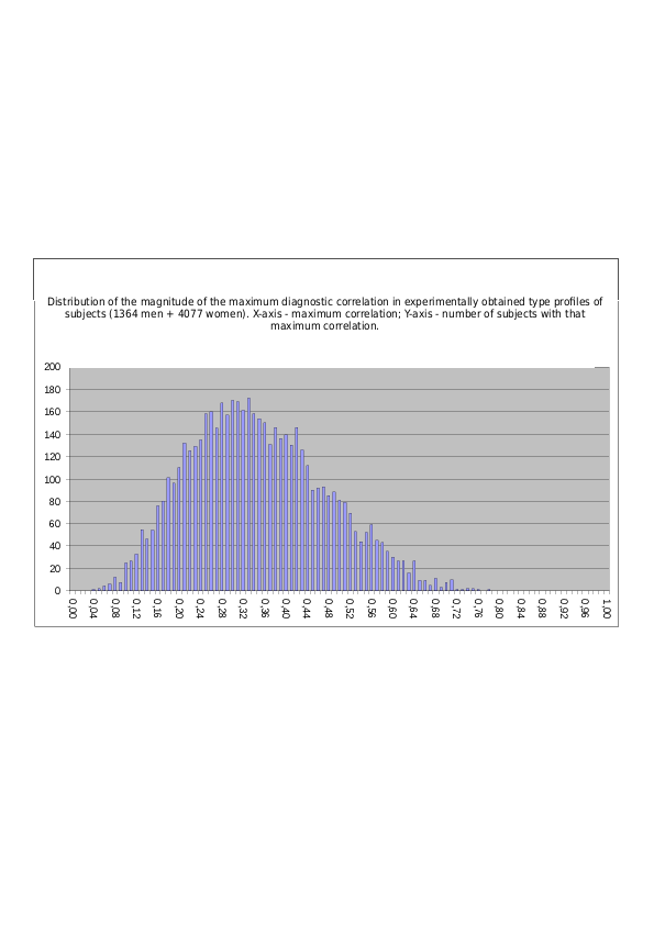
Below, in Figs. 1.1-1.3, distributions are shown for the magnitude of the maximum experimentally obtained diagnostic correlation (the maximum correlation in the subjects’ experimentally obtained type profiles) in the experimental sample consisting of 1364 men and 4077 women. The broad differences in the magnitude of the maximum correlation (as a rule, found with the one most suitable among all 16 standard types) reflect very substantial interindividual differences in the proportion of influence exerted specifically by factors of socionic temperament on subjects’ questionnaire answers. People with low correlation coefficients (even provided that this is the maximum correlation coefficient in their type profile) evidently either give careless and hasty answers to the questionnaire questions or simply have poor ability to evaluate themselves in comparison with other people. It is true that in most cases their maximum correlation coefficient with one of the types (even if low in absolute value) nevertheless correctly indicates their type, owing to the large number of questionnaire questions. However, for quantitative comparison of their results with the results of other subjects (who provide more reliable answers and therefore show higher correlation coefficients), the results of all subjects must be brought to the same scale, which is the purpose of the operation of normalizing type profiles, performed by the above-described Method No. 1 or Method No. 2. Another noteworthy fact is that women on average provide less reliable answers than men (mean maximum profile correlation 0,345 versus 0,352 in men) – there are, however, two exceptions to this rule: in the separate subsample of irrational types and the separate subsample of extraverts, women provide more reliable results (with higher mean correlation coefficients) than men. In addition, women as a whole are more psychologically homogeneous across the entire sample and, in particular, differ less from one another in answer reliability than men (distribution half-width 0,125 in women versus 0,135 in men; here, qualitative differences between the subsamples of extraverts and introverts, rationals and irrationals, etc., are no longer found). The distributions shown in the diagrams of Figs. 1.1-1.3 indicate that the proportion of influence exerted specifically by socionic factors on subjects’ answers to the psychological questionnaire (that is, the corresponding proportion of influence on the total variance of those answers) ranges across different subjects from 0,2% to 60%, and averages approximately 12% across the sample (the square of the mean correlation coefficient multiplied by 100%). This comparatively small proportion of influence exerted by psychophysiological temperament associated with socionics on the answers nevertheless proves entirely sufficient for reliable type diagnosis of subjects. Moreover - in most cases, constructing a type profile composed of diagnostic correlations reliably diagnoses not only the primary sociotype but also an additional socionic accentuation in the subjects.
Fig. 1.1. Distribution of the magnitude of the maximum diagnostic correlation in the experimentally obtained type profiles of subjects (1364 men). Mean value of the maximum correlation = 0,352; standard deviation (half-width of the distribution) = 0,135.
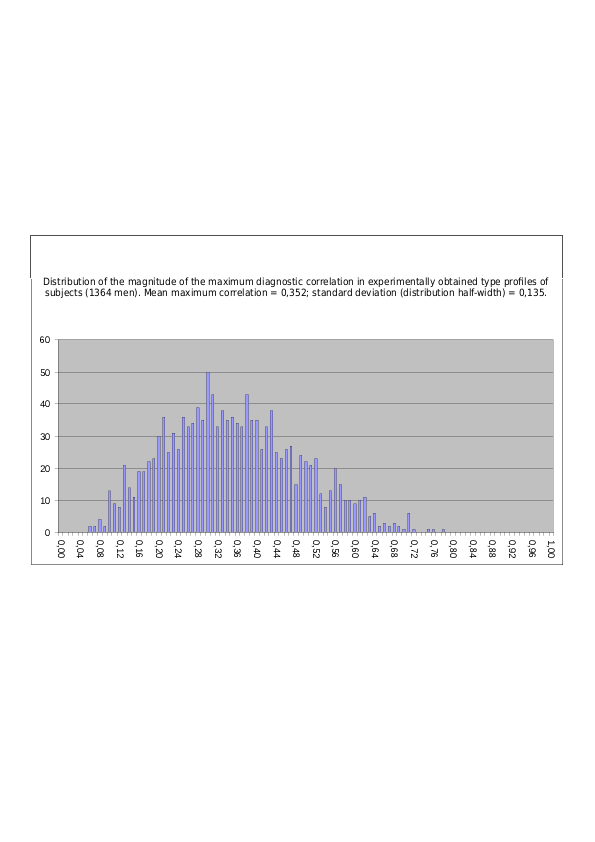
Fig. 1.2. Distribution of the magnitude of the maximum diagnostic correlation in the experimentally obtained type profiles of subjects (4077 women). Mean value of the maximum correlation = 0,345; standard deviation (half-width of the distribution) = 0,125.
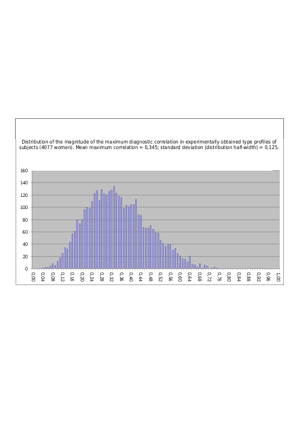
Fig. 1.3. Distribution of the magnitude of the maximum diagnostic correlation in the experimentally obtained type profiles of subjects (1364 men + 4077 women). X-axis - magnitude of the maximum correlation; Y-axis - number of subjects with such a maximum correlation.
Part 1 – Boundaries Between Psychotypes
Results of the Study of Boundaries Between Psychotypes - Provided That the Subjects’ Type Profile Is Composed of Diagnostic Correlations
In this section we shall present graphical representations (diagrams) of the boundaries between psychotypes (obtained empirically) for both variants of normalization of the primary diagnostic correlations – both by Method No. 1 and by Method No. 2. We perform this “double work” so that no doubts remain about the validity of the results and the conclusions based on them.
The scientific question to which we wish to find an answer is the following: do objective boundaries between sociotypes exist? If there are no boundaries, then in subjects’ type profiles (composed of diagnostic correlations between their questionnaire answers and the reference answers of the 16 psychotypes), the number of cases in which two profile correlations simultaneously reach practically the same maximum will be substantial – these are precisely the cases in which subjects, by their properties, lie strictly on the boundary between two socionic types. The experimental material presented below shows, however, that objective boundaries do exist – although they are somewhat blurred (blurred - especially between quasi-identical types, which are the closest to one another in psychological properties). This means that most subjects gravitate toward one of the two types, including quasi-identical types, while at the same time a comparatively small percentage of subjects are found whose properties place them almost exactly on the boundary between two types. That is, this boundary is objectively marked, but it is not entirely empty, that is, it is blurred. The boundary between types that are still more distant from one another in their properties (for example, between ILI and ILE and other types in the so-called socionic relations of complete opposition, or between mirror types, ILI and LIE, etc.) is expressed much more clearly, but it too is not perfectly empty. The boundary between conflict types (those differing most strongly in their properties), however, is already completely empty, free even of individual subjects in its vicinity.
In drawing a conclusion from the experimental material presented below that objective boundaries between socionic types exist, some caution must nevertheless be observed. The point is that the apparatus of diagnostic correlations is an apparatus of a kind of filters, selectively tuned in their transmission – neither to the left nor to the right! - to particular zones of psychological space (which we call psychotypes). This selective tuning of the filters can generate an artifact of apparently, supposedly objectively existing boundaries that are, however, absent at the level of physiological parameters and are fictitious. As an example, recall the decomposition of the continuous spectrum of daylight into a rainbow by means of a prism – in the resulting rainbow image, the human eye rather confidently distinguishes 7 local zones, albeit with blurred boundaries – violet, blue, light blue, green, yellow, orange, and red. This, however, does not imply that these 7 bulges are objectively present in the spectrum of sunlight – unfortunately, it is smooth and continuous. The illusion of eight separated color zones arises only because our eye has three selective color detectors - the blue-sensitive, green-sensitive, and red-sensitive cones of the retina.
The objective nature of boundaries between psychotypes can be judged with greater confidence from the results of those experiments (also presented below in Part 2 of the article) in which bipolarity is revealed in the distribution of subjects along the extraversion-introversion, intuition-sensing, and logic-ethics axes. The point is that the corresponding indices are calculated not using a single filter in the form of one diagnostic correlation selectively tuned to a psychotype, but using the sum of the passbands of several such filters at once (in the form of the sum of the diagnostic correlations of all extraverted types, for example, to determine the magnitude of individual extraversion). Looking ahead, we note that these results also confirm the existence of objective boundaries – the distribution of people along the indicated axes proves bipolar, although the boundary between the poles is not absolutely empty. Still greater weight for conclusions about the objectivity of boundaries between psychotypes is provided by the distribution of the magnitudes of all 8 socionic functions combined in a single diagram (see Part 3 of the article) – this distribution proves noticeably multimodal (especially among men), indicating that certain specific magnitudes are preferred for socionic functions in the population, that is, they are partly – albeit diffusely – quantized, which testifies to the comparatively separate existence of the types from one another.
For a more precise and final conclusion about the separation from one another (at least partial separation) of the poles of the three basic socionic traits and the mutual separation of psychotypes (especially quasi-identical ones), however, additional experiments are required in which the quantities of interest would be diagnosed not by locally and selectively tuned filters in the form of diagnostic correlations, but by so-called continuous diagnostic scales. Such a study is entirely feasible on the basis of the experimental material we have already collected, but it requires a complete, fundamental recalculation on a different basis and has therefore been planned by us for the future.
Boundaries Between QUASI-IDENTICAL Types - with Diagnostic Correlations Normalized by Method No. 1
Fig. 2.1. Population distribution of the difference between normalized diagnostic correlations (normalization by Method No. 1) between the type diagnosed in subjects (the “primary type”) and its quasi-identical type (ILI for LII, LII for ILI, LSE for SLE, SLE for LSE, etc.; 16 possible differences in total for 16 pairs of types). Male sample.
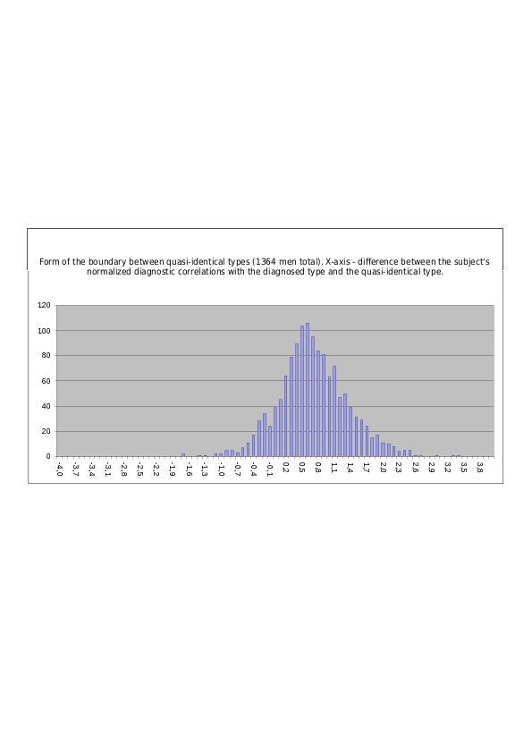
Fig. 2.2. Population distribution of the difference between normalized diagnostic correlations (normalization by Method No. 1) between the type diagnosed in subjects (the “primary type”) and its quasi-identical type (ILI for LII, LII for ILI, LSE for SLE, SLE for LSE, etc.; 16 possible differences in total for 16 pairs of types). Female sample.
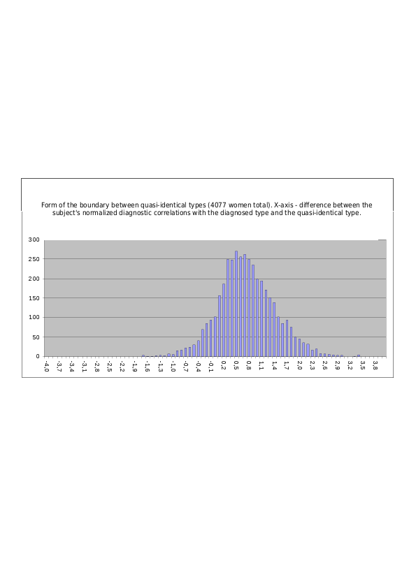
Fig. 2.3. Population distribution of the difference between normalized diagnostic correlations (normalization by Method No. 1) between the type diagnosed in subjects (the “primary type”) and its quasi-identical type (ILI for LII, LII for ILI, LSE for SLE, SLE for LSE, etc.; 16 possible differences in total for 16 pairs of types). Mixed sample. The relative density of subjects located exactly on the boundary between the types (the case in which the difference between diagnostic correlations =0) is 38% of the maximum density (=141/374*100%). The transition from one type to the other is therefore smooth and continuous, although the boundary between the types is nevertheless visible in the decline in the probability density of finding subjects on it.
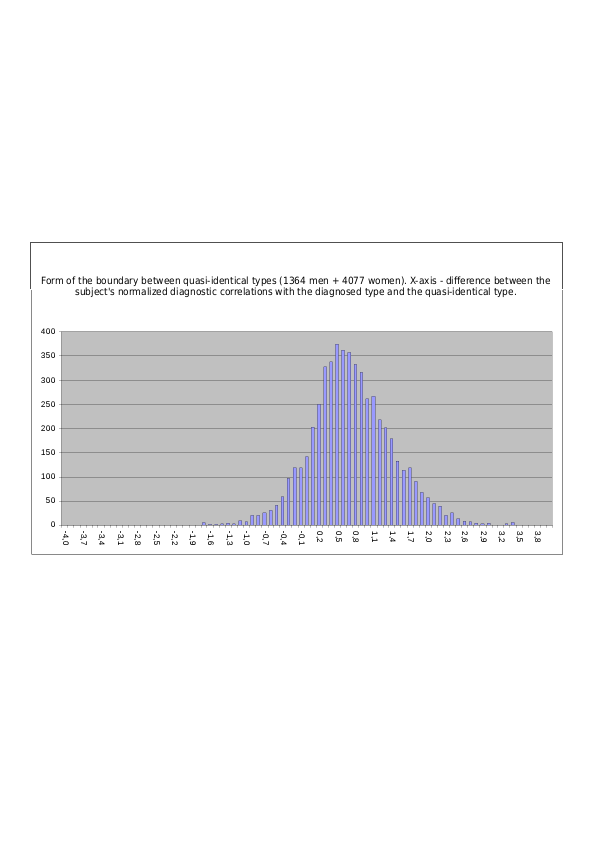
Fig. 2.4. Population distribution of the difference between normalized diagnostic correlations (normalization by Method No. 1) between the type diagnosed in subjects (the “primary type”) and its quasi-identical type, plus between the quasi-identical and primary types (yielding 32 possible differences in total for 16 pairs of types). Mixed sample. The relative density of subjects located exactly on the boundary between the types (the case in which the difference between diagnostic correlations =0) is approximately 66% (282/425*100%=66%) of the maximum density found at the center of each psychotype in the pair. Compared with the preceding figure, the relative boundary density has increased almost twofold because here the possibility that the subject belongs to either one or the other type in the pair is taken into account – as a result, the absolute density at the boundary between them doubles, while the probability of finding a subject at the center of each peak increases only slightly because it is summed with the declining flank from the other peak. The transition from one type to the other is smooth and continuous, although the boundary between the types is nevertheless visible in the decline in the probability density of finding subjects on it.
Boundaries Between QUASI-IDENTICAL Types with Diagnostic Correlations Normalized by Method No. 2
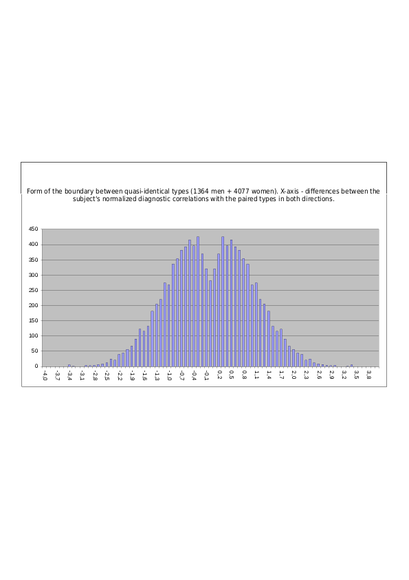
Fig. 2.5. Population distribution of the difference between normalized diagnostic correlations (normalization of the empirical correlations of subjects’ type profiles by Method No. 2) between the type diagnosed in subjects (the “primary type”) and its quasi-identical type (ILI for LII, LII for ILI, LSE for SLE, SLE for LSE, etc.; 16 possible differences in total for 16 pairs of types). Mixed sample. The relative density of subjects located exactly on the boundary between the types (the case in which the difference between diagnostic correlations =0) is 29% of the maximum density (=138/472*100%), that is, it is far from zero. The maximum density of subjects corresponds to the normalized diagnostic correlation of the quasi-identical type lagging behind the normalized diagnostic correlation of the primary diagnosed type in the type profile by 0,50 (on the scale of diagnostic correlations normalized by Method No. 2). The transition from one type to the other is therefore smooth and continuous, although the boundary between the types is nevertheless visible in the decline in the probability density of finding subjects on it.
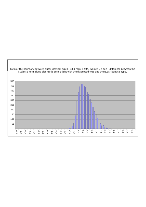
Fig. 2.6. Population distribution of the difference between normalized diagnostic correlations (normalization by Method No. 2) between the type diagnosed in subjects (the “primary type”) and its quasi-identical type, plus between the quasi-identical and primary types (the diagram combines 32 possible differences in total for 16 pairs of types). Mixed sample. The relative density of subjects located exactly on the boundary between the types (the case in which the difference between diagnostic correlations =0) is approximately 58% (276/476*100%=58%) of the maximum density found at the center of each psychotype in the pair. Compared with the preceding figure, the relative boundary density has doubled because here the possibility that the subject belongs to either one or the other type in the pair is taken into account – as a result, the absolute density at the boundary between them doubles, while the probability of finding a subject at the center of each peak increases only slightly because it is summed with the declining flank from the other peak. The transition from one type to the other is smooth and continuous, although the boundary between the types is nevertheless visible in the decline in the probability density of finding subjects on it.
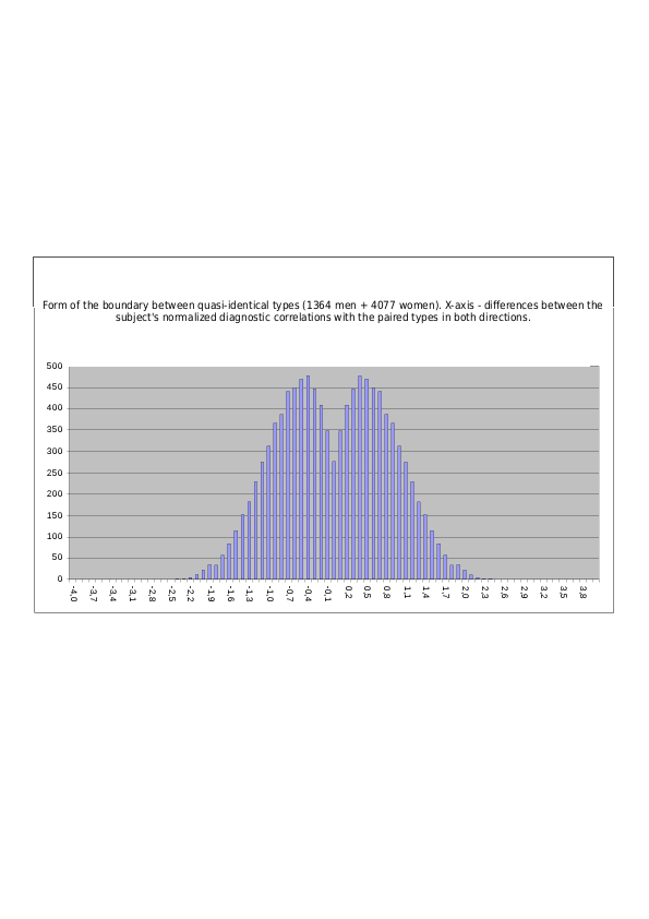
Boundaries Between KINDRED Types with Diagnostic Correlations Normalized by Method No. 1
Fig. 3.1. Population distribution of the difference between normalized diagnostic correlations (normalization by Method No. 1) between the type diagnosed in subjects (the “primary type”) and its kindred type (IEE for ILE, ILE for IEE, LSI for LII, LII for LSI, etc.; 16 possible differences in total for 16 pairs of types). Male sample.
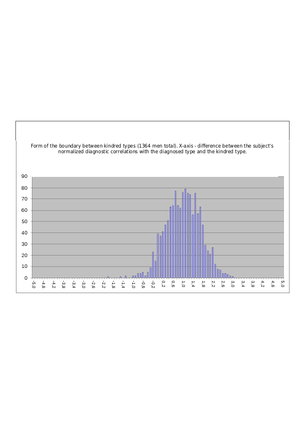
Fig. 3.2. Population distribution of the difference between normalized diagnostic correlations (normalization by Method No. 1) between the type diagnosed in subjects (the “primary type”) and its kindred type (IEE for ILE, ILE for IEE, LSI for LII, LII for LSI, etc.; 16 possible differences in total for 16 pairs of types). Female sample.
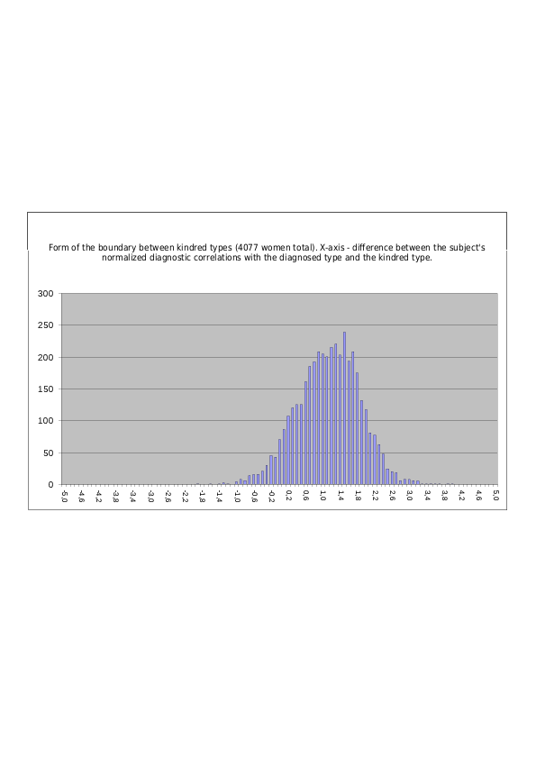
Fig. 3.3. Population distribution of the difference between normalized diagnostic correlations (normalization by Method No. 1) between the type diagnosed in subjects (the “primary type”) and its kindred type (IEE for ILE, ILE for IEE, LSI for LII, LII for LSI, etc.; 16 possible differences in total for 16 pairs of types). Mixed sample. The relative density of subjects located exactly on the boundary between the types (the case in which the difference between diagnostic correlations =0) is 33% of the maximum density (=100/300*100%). The transition from one type to the other is smooth and continuous, although the boundary between the types is nevertheless clearly visible in the decline in the probability density of finding subjects on it.
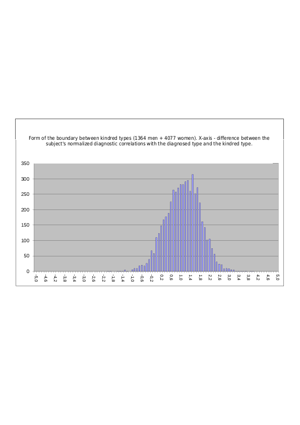
Fig. 3.4. Population distribution of the difference between normalized diagnostic correlations (normalization by Method No. 1) between the type diagnosed in subjects (the “primary type”) and its kindred type, plus between the kindred and primary types (the diagram combines 32 differences in total for 16 pairs of types). Mixed sample. The relative density of subjects located exactly on the boundary between the types (the case in which the difference between diagnostic correlations =0) is approximately 63% (200/315*100%=63%) of the maximum density found at the center of each psychotype in the pair. Compared with the preceding figure, the boundary density has increased approximately twofold because here the possibility that the subject belongs to either one or the other type in the pair is taken into account – as a result, the density at the boundary between them doubles. The transition from one type to the other is smooth and continuous, although the boundary between the types is nevertheless clearly visible in the decline in the probability density of finding subjects on it.
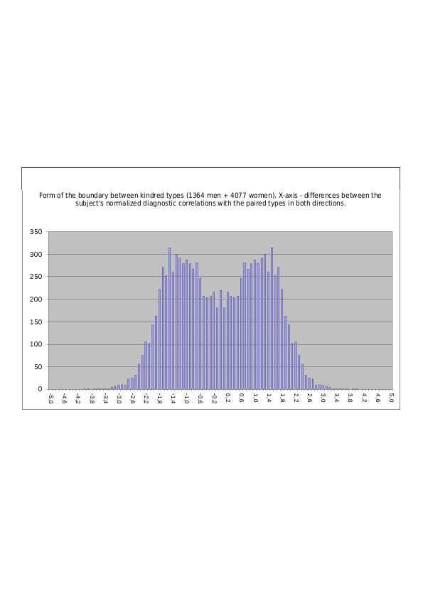
Boundaries Between KINDRED Types with Diagnostic Correlations Normalized by Method No. 2
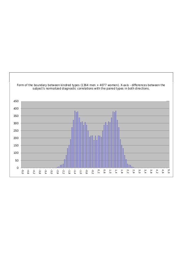
Fig. 3.5. Population distribution of the difference between normalized diagnostic correlations (normalization by Method No. 2) between the type diagnosed in subjects (the “primary type”) and its kindred type (IEE for ILE, ILE for IEE, LSI for LII, LII for LSI, etc.; 16 possible differences in total for 16 pairs of types). Mixed sample. The relative density of subjects located exactly on the boundary between the types (the case in which the difference between diagnostic correlations =0) is approximately 28% of the maximum density (=108/383*100%). The transition from one type to the other is smooth and continuous, although the boundary between the types is nevertheless clearly visible in the decline in the probability density of finding subjects on it.
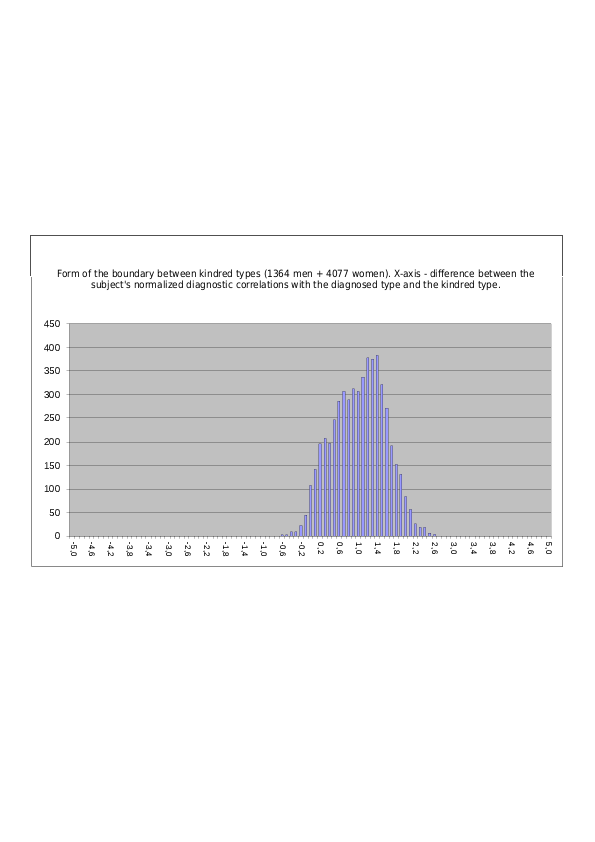
Fig. 3.6. Population distribution of the difference between normalized diagnostic correlations (normalization by Method No. 2) between the type diagnosed in subjects (the “primary type”) and its kindred type, plus between the kindred and primary types (the diagram combines 32 differences in total for 16 pairs of types). Mixed sample. The relative density of subjects located exactly on the boundary between the types (the case in which the difference between diagnostic correlations =0) is approximately 56% (216/383*100%=56%) of the maximum density found at the center of each psychotype in the pair. Compared with the preceding figure, the boundary density has increased approximately twofold because here the possibility that the subject belongs to either one or the other type in the pair is taken into account – as a result, the density at the boundary between them doubles. The transition from one type to the other is smooth and continuous, although the boundary between the types is nevertheless clearly visible in the decline in the probability density of finding subjects on it.
Boundaries Between Types in BUSINESS RELATIONS with Diagnostic Correlations Normalized by Method No. 1
Fig. 4.1. Population distribution of the difference between normalized diagnostic correlations (normalization by Method No. 1) between the type diagnosed in subjects (the “primary type”) and the type in a Business relation with it (SLE for ILE, ILE for SLE, EII for LII, LII for EII, etc.; 16 possible differences in total for 16 pairs of types). Male sample.
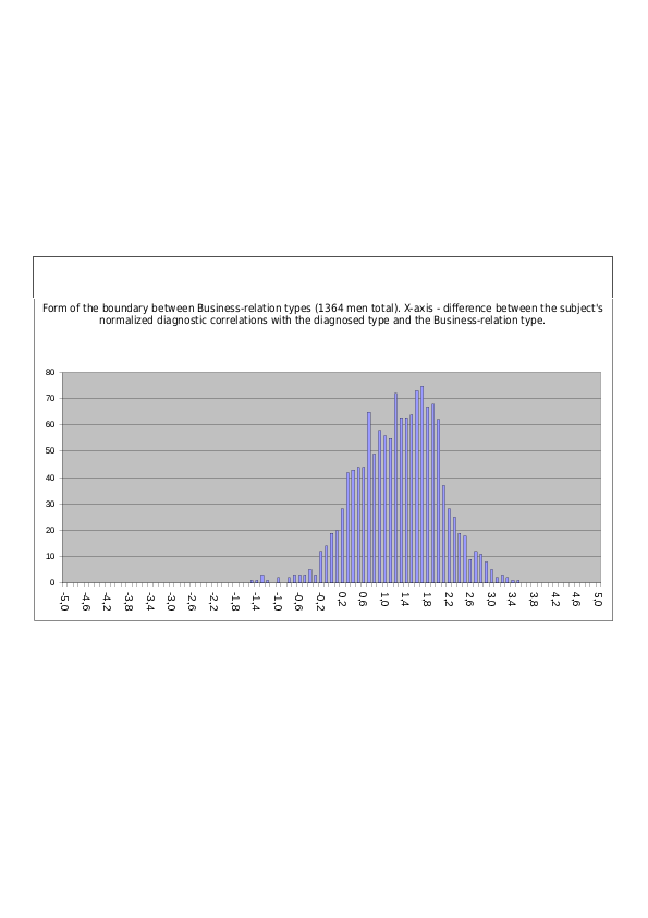
Fig. 4.2. Population distribution of the difference between normalized diagnostic correlations (normalization by Method No. 1) between the type diagnosed in subjects (the “primary type”) and the type in a Business relation with it (SLE for ILE, ILE for SLE, EII for LII, LII for EII, etc.; 16 possible differences in total for 16 pairs of types). Female sample.
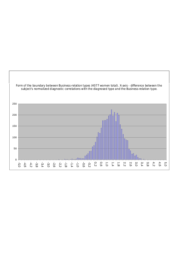
Fig. 4.3. Population distribution of the difference between normalized diagnostic correlations (normalization by Method No. 1) between the type diagnosed in subjects (the “primary type”) and the type in a Business relation with it (SLE for ILE, ILE for SLE, EII for LII, LII for EII, etc.; 16 possible differences in total for 16 pairs of types). Mixed sample. The relative density of subjects located exactly on the boundary between the types (the case in which the difference between diagnostic correlations =0) is approximately 26% of the maximum density (=76/287*100%). The transition from one type to the other remains formally smooth and continuous, although the boundary between the types is nevertheless clearly visible from the sharp decline in the probability density of finding subjects on it.
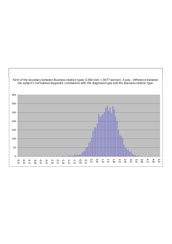
Fig. 4.4. Population distribution of the difference between normalized diagnostic correlations (normalization by Method No. 1) between the type diagnosed in subjects (the “primary type”) and the type in a Business relation with it, plus between the Business-related and primary types (the diagram combines 32 differences in total for 16 pairs of types). Mixed sample. The relative density of subjects located exactly on the boundary between the types (the case in which the difference between diagnostic correlations =0) is approximately 52% (150/291*100%=52%) of the maximum density found at the center of each psychotype in the pair. Compared with the preceding figure, the boundary density has increased approximately twofold because here the possibility that the subject belongs to either one or the other type in the pair is taken into account – as a result, the density at the boundary between them doubles. The transition from one type to the other remains formally smooth and continuous, although the boundary between the types is nevertheless clearly visible from the sharp decline in the probability density of finding subjects on it.
Boundaries Between Types in BUSINESS RELATIONS with Diagnostic Correlations Normalized by Method No. 2
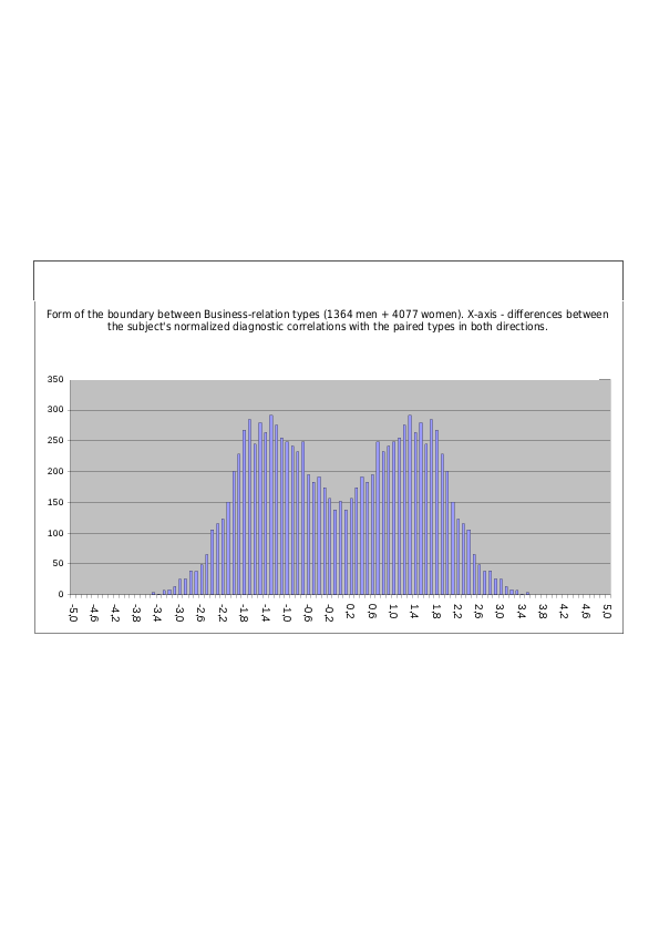
Fig. 4.5. Population distribution of the difference between normalized diagnostic correlations (normalization by Method No. 2) between the type diagnosed in subjects (the “primary type”) and the type in a Business relation with it (SLE for ILE, ILE for SLE, EII for LII, LII for EII, etc.; 16 possible differences in total for 16 pairs of types). Mixed sample. The relative density of subjects located exactly on the boundary between the types (the case in which the difference between diagnostic correlations =0) is approximately 22% of the maximum density (=80/359*100%). The transition from one type to the other remains smooth and continuous, although the boundary between the types is clearly visible from the sharp decline in the probability density of finding subjects on it.
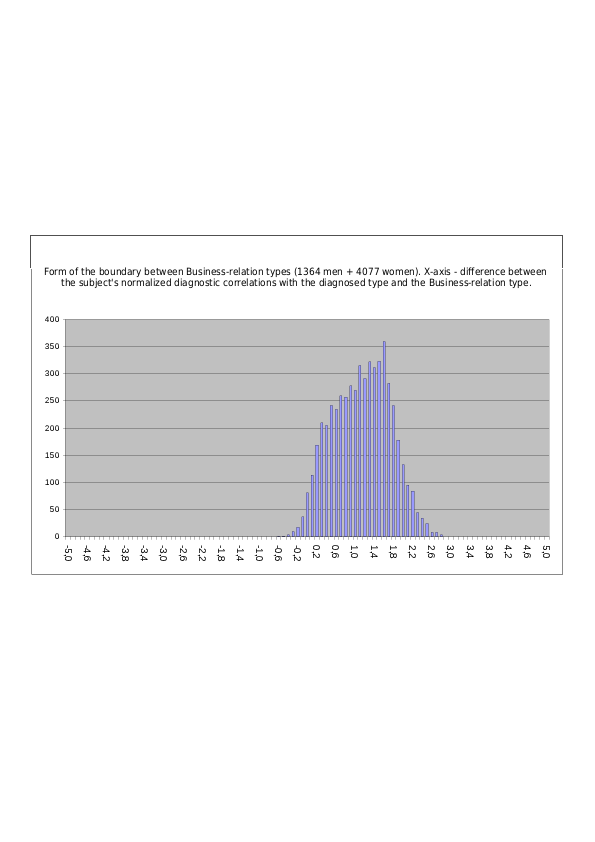
Fig. 4.6. Population distribution of the difference between normalized diagnostic correlations (normalization by Method No. 2) between the type diagnosed in subjects (the “primary type”) and the type in a Business relation with it, plus between the Business-related and primary types (the diagram combines 32 differences in total for 16 pairs of types). Mixed sample. The relative density of subjects located exactly on the boundary between the types (the case in which the difference between diagnostic correlations =0) is approximately 44% (160/359*100%=43%) of the maximum density found at the center of each psychotype in the pair. Compared with the preceding figure, the boundary density has doubled because here the possibility that the subject belongs to either one or the other type in the pair is taken into account – as a result, the density at the boundary between them doubles. The transition from one type to the other remains smooth and continuous, although the boundary between the types is clearly visible from the sharp decline in the probability density of finding subjects on it.
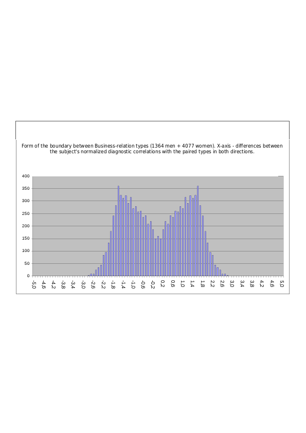
Boundaries Between Types in COMPLETE OPPOSITION Relations, with Diagnostic Correlations Normalized by Method No. 1
Fig. 5.1. Population distribution of the difference between normalized diagnostic correlations (normalization by Method No. 1) between the type diagnosed in subjects (the “primary type”) and the type in a complete opposition relation with it (ILI for ILE, ILE for ILI, LIE for LII, LII for LIE, etc.; 16 possible differences in total for 16 pairs of types). Male sample.
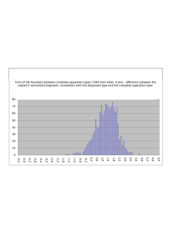
Fig. 5.2. Population distribution of the difference between normalized diagnostic correlations (normalization by Method No. 1) between the type diagnosed in subjects (the “primary type”) and the type in a complete opposition relation with it (ILI for ILE, ILE for ILI, LIE for LII, LII for LIE, etc.; 16 possible differences in total for 16 pairs of types). Female sample.
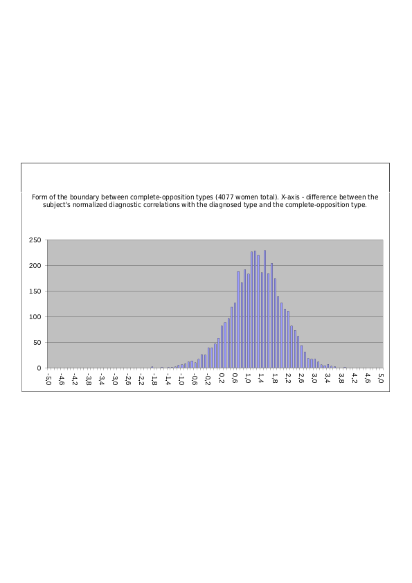
Fig. 5.3. Population distribution of the difference between normalized diagnostic correlations (normalization by Method No. 1) between the type diagnosed in subjects (the “primary type”) and the type in a complete opposition relation with it (ILI for ILE, ILE for ILI, LIE for LII, LII for LIE, etc.; 16 possible differences in total for 16 pairs of types). Mixed sample. The relative density of subjects located exactly on the boundary between the types (the case in which the difference between diagnostic correlations =0) is approximately 22% (=65/301*100%) of the maximum density found at the center of the psychotype. The transition from one type to the other remains smooth and continuous; the boundary is not empty, and individual accentuated cases from the population are present on it, although the boundary between the types is nevertheless clearly visible from the sharp decline in the probability density of finding subjects on it.
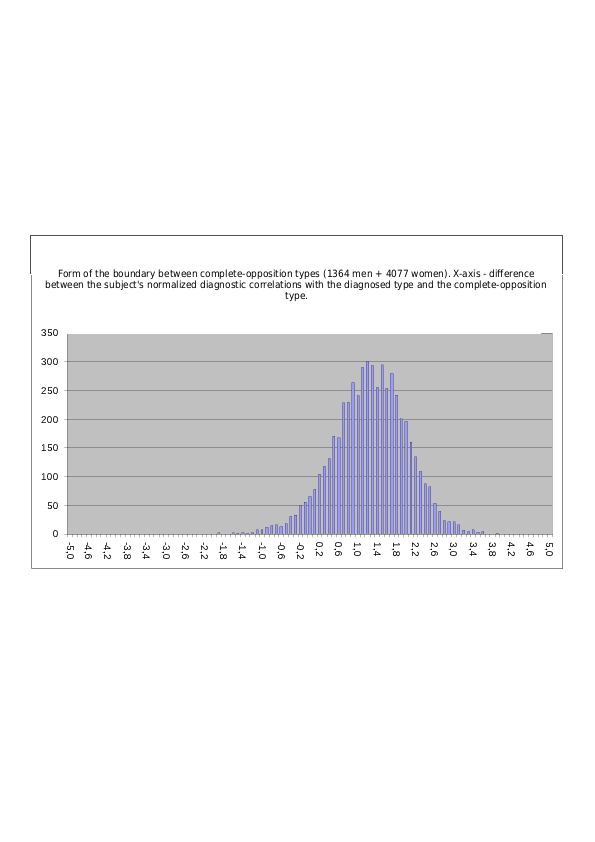
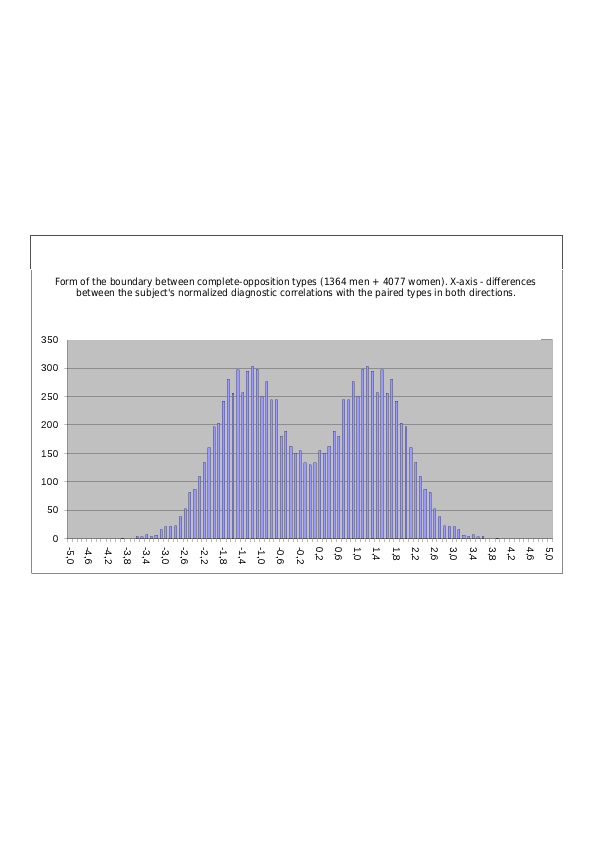
Fig. 5.4. Population distribution of the difference between normalized diagnostic correlations (normalization by Method No. 1) between the type diagnosed in subjects (the “primary type”) and the type in a complete opposition relation with it, plus between the type in a complete opposition relation and the primary type (the diagram combines 32 possible differences in total for 16 pairs of types). Mixed sample. The relative density of subjects located exactly on the boundary between the types (the case in which the difference between diagnostic correlations =0) is approximately 43% (130/303*100%=43%) of the maximum density found at the center of each psychotype in the pair. Compared with the preceding figure, the boundary density has increased approximately twofold because here the possibility that the subject belongs to either one or the other type in the pair is taken into account – as a result, the density at the boundary between them doubles. The transition from one type to the other remains smooth and continuous; the boundary is not empty, and individual accentuated cases from the population are present on it, although the boundary between the types is nevertheless clearly visible from the sharp decline in the probability density of finding subjects on it.
Boundaries Between Types in COMPLETE OPPOSITION Relations, with Diagnostic Correlations Normalized by Method No. 2
Fig. 5.5. Population distribution of the difference between normalized diagnostic correlations (normalization by Method No. 2) between the type diagnosed in subjects (the “primary type”) and the type in a complete opposition relation with it (ILI for ILE, ILE for ILI, LIE for LII, LII for LIE, etc.; 16 possible differences in total for 16 pairs of types). Mixed sample. The relative density of subjects located exactly on the boundary between the types (the case in which the difference between diagnostic correlations =0) is approximately 15% (=58/397*100%) of the maximum density found at the center of the psychotype. The transition from one type to the other remains smooth and continuous; the boundary is not empty, and individual accentuated cases from the population are present on it, although the boundary between the types is nevertheless clearly visible from the sharp decline in the probability density of finding subjects on it.
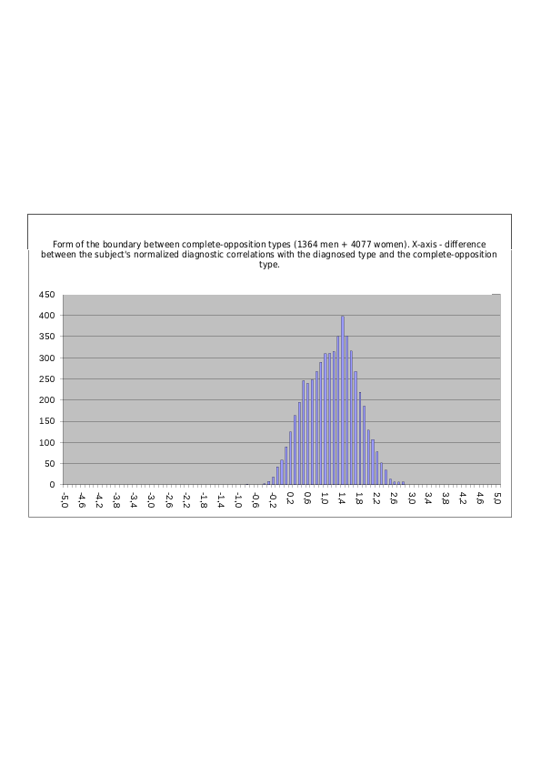
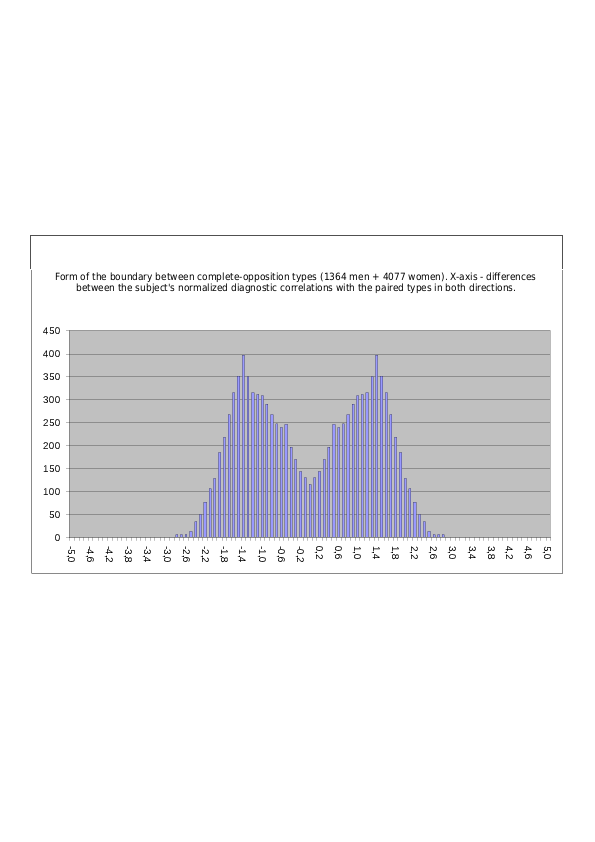
Fig. 5.6. Population distribution of the difference between normalized diagnostic correlations (normalization by Method No. 2) between the type diagnosed in subjects (the “primary type”) and the type in a complete opposition relation with it, plus between the type in a complete opposition relation and the primary type (the diagram combines 32 possible differences in total for 16 pairs of types). Mixed sample. The relative density of subjects located exactly on the boundary between the types (the case in which the difference between diagnostic correlations =0) is approximately 29% (116/397*100%=29%) of the maximum density found at the center of each psychotype in the pair. Compared with the preceding figure, the boundary density has doubled because here the possibility that the subject belongs to either one or the other type in the pair is taken into account – as a result, the density at the boundary between them doubles. The transition from one type to the other remains smooth and continuous; the boundary is not empty, and individual accentuated cases from the population are present on it, although the boundary between the types is nevertheless clearly visible from the sharp decline in the probability density of finding subjects on it.
Boundaries Between Types in MIRROR Relations, with Diagnostic Correlations Normalized by Method No. 1
Fig. 6.1. Population distribution of the difference between normalized diagnostic correlations (normalization by Method No. 1) between the type diagnosed in subjects (the “primary type”) and the type in a Mirror relation with it (LII for ILE, ILE for LII, ESE for SEI, SEI for ESE, etc.; 16 possible differences in total for 16 pairs of types). Male sample.
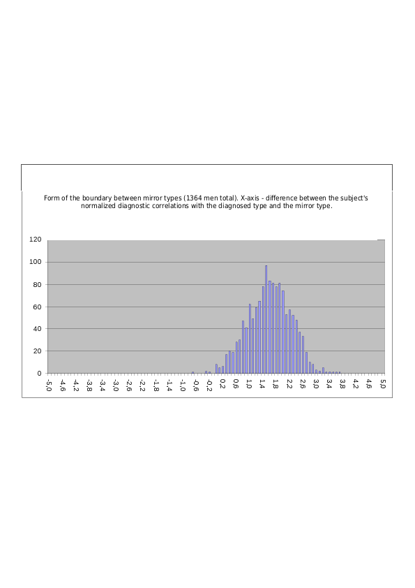
Fig. 6.2. Population distribution of the difference between normalized diagnostic correlations (normalization by Method No. 1) between the type diagnosed in subjects (the “primary type”) and the type in a Mirror relation with it (LII for ILE, ILE for LII, ESE for SEI, SEI for ESE, etc.; 16 possible differences in total for 16 pairs of types). Female sample.
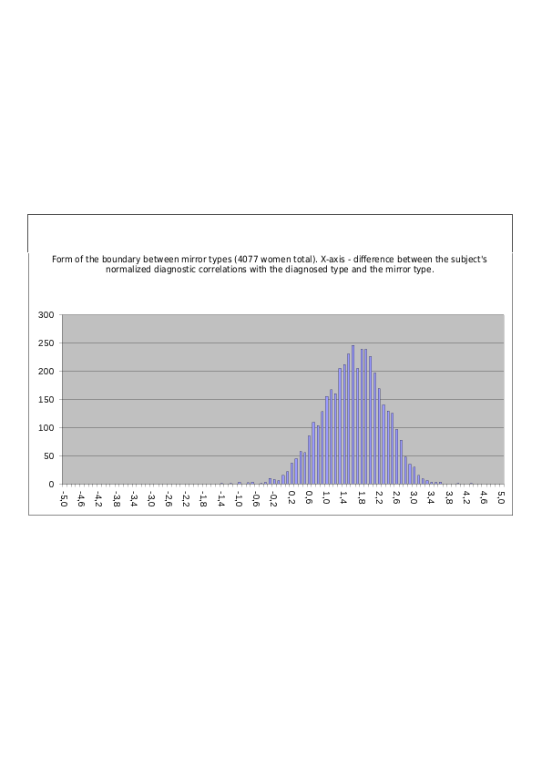
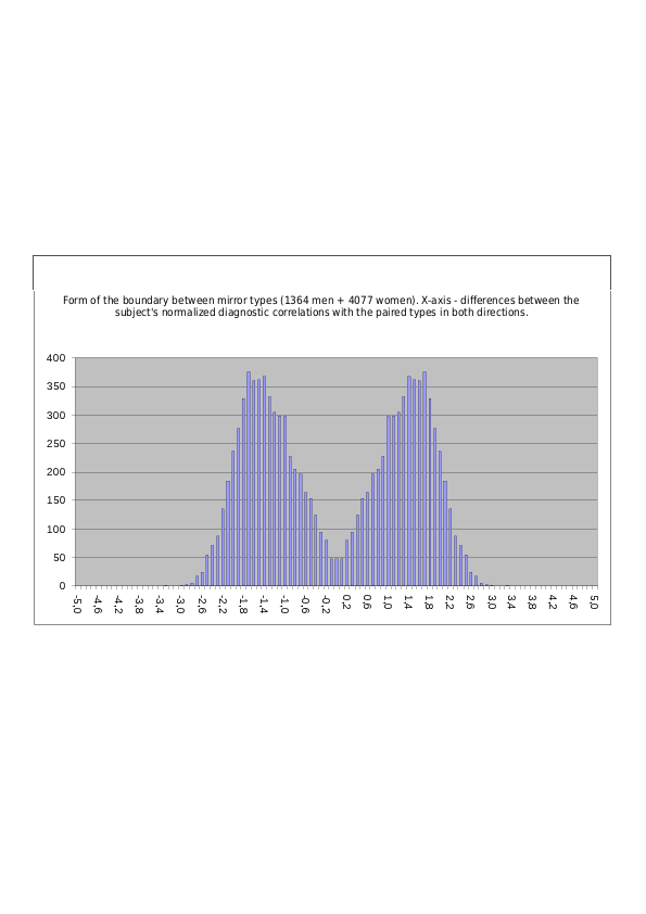
Fig. 6.3. Population distribution of the difference between normalized diagnostic correlations (normalization by Method No. 1) between the type diagnosed in subjects (the “primary type”) and the type in a Mirror relation with it (LII for ILE, ILE for LII, ESE for SEI, SEI for ESE, etc.; 16 possible differences in total for 16 pairs of types). Mixed sample. The relative density of subjects located exactly on the boundary between the types (the case in which the difference between diagnostic correlations =0) is approximately 7% (=23/329*100%) of the maximum density found at the center of the psychotype. The transition from one type to the other remains smooth and continuous; the boundary is not empty, and individual accentuated cases from the population are present on it, although the boundary between the types is nevertheless clearly visible from the sharp decline in the probability density of finding subjects on it.
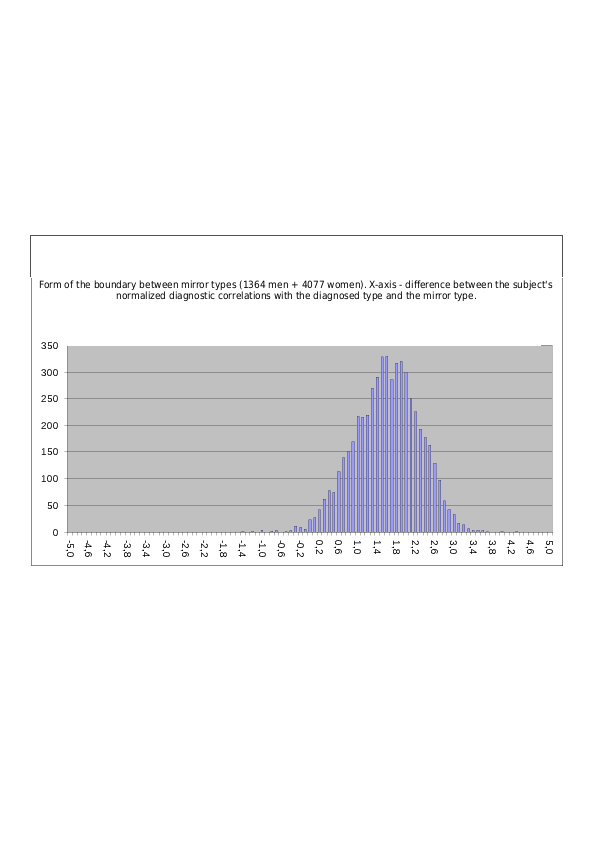
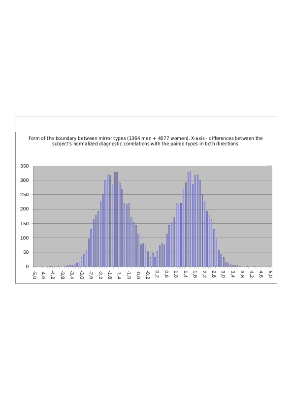
Fig. 6.4. Population distribution of the difference between normalized diagnostic correlations (normalization by Method No. 1) between the type diagnosed in subjects (the “primary type”) and the type in a Mirror relation with it, plus conversely between the mirror type and the subject’s primary type (the diagram combines 32 possible differences in total for 16 pairs of types). Mixed sample. The relative density of subjects located exactly on the boundary between the types (the case in which the difference between diagnostic correlations =0) is approximately 14% (46/329*100%=14%) of the maximum density found at the center of each psychotype in the pair. Compared with the preceding figure, the boundary density has doubled because here the possibility that the subject belongs to either one or the other type in the pair is taken into account – as a result, the density at the boundary between them doubles. The transition from one type to the other remains smooth and continuous; the boundary is not empty, and individual accentuated cases from the population are present on it, although the boundary between the types is nevertheless clearly visible from the sharp, nearly to zero, decline in the probability density of finding subjects on it.
Boundaries Between Types in MIRROR Relations, with Diagnostic Correlations Normalized by Method No. 2
Fig. 6.5. Population distribution of the difference between normalized diagnostic correlations (normalization by Method No. 2) between the type diagnosed in subjects (the “primary type”) and the type in a Mirror relation with it (LII for ILE, ILE for LII, ESE for SEI, SEI for ESE, etc.; 16 possible differences in total for 16 pairs of types). Mixed sample. The relative density of subjects located exactly on the boundary between the types (the case in which the difference between diagnostic correlations =0) is approximately 6% (=24/376*100%) of the maximum density found at the center of the psychotype. The transition from one type to the other remains smooth and continuous; the boundary is not empty, and individual accentuated cases from the population are present on it, although the boundary between the types is nevertheless clearly visible from the sharp decline in the probability density of finding subjects on it.
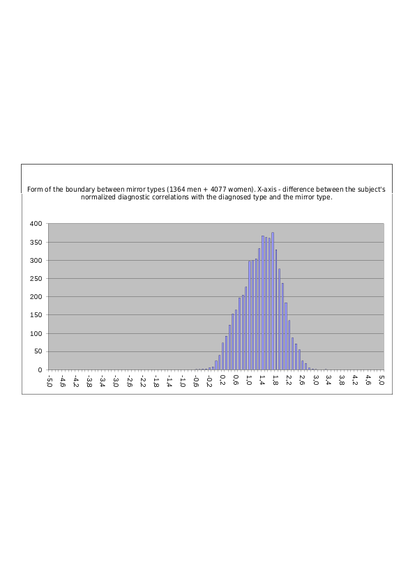
Fig. 6.6. Population distribution of the difference between normalized diagnostic correlations (normalization by Method No. 2) between the type diagnosed in subjects (the “primary type”) and the type in a Mirror relation with it, plus conversely between the mirror type and the subject’s primary type (the diagram combines 32 possible differences in total for 16 pairs of types). Mixed sample. The relative density of subjects located exactly on the boundary between the types (the case in which the difference between diagnostic correlations =0) is approximately 13% (48/376*100%) of the maximum density found at the center of each psychotype in the pair. Compared with the preceding figure, the boundary density has doubled because here the possibility that the subject belongs to either one or the other type in the pair is taken into account – as a result, the density at the boundary between them doubles. The transition from one type to the other remains smooth and continuous; the boundary is not empty, and individual accentuated cases from the population are present on it, although the boundary between the types is nevertheless clearly visible from the sharp, nearly to zero, decline in the probability density of finding subjects on it.
Boundaries Between Types in CONFLICT Relations, with Diagnostic Correlations Normalized by Method No. 1
Fig. 7.1. Population distribution of the difference between normalized diagnostic correlations (normalization by Method No. 1) between the type diagnosed in subjects (the “primary type”) and the type in a CONFLICT relation with it (ESI for ILE, ILE for ESI, SEE for LII, LII for SEE, etc.; 16 differences in total for 16 pairs of types). Male sample.
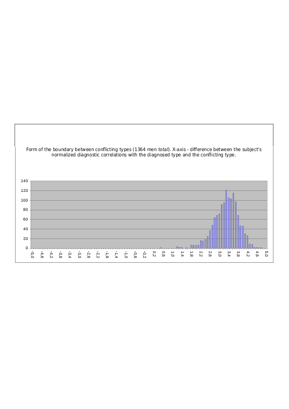
Fig. 7.2. Population distribution of the difference between normalized diagnostic correlations (normalization by Method No. 1) between the type diagnosed in subjects (the “primary type”) and the type in a CONFLICT relation with it (ESI for ILE, ILE for ESI, SEE for LII, LII for SEE, etc.; 16 differences in total for 16 pairs of types). Female sample.
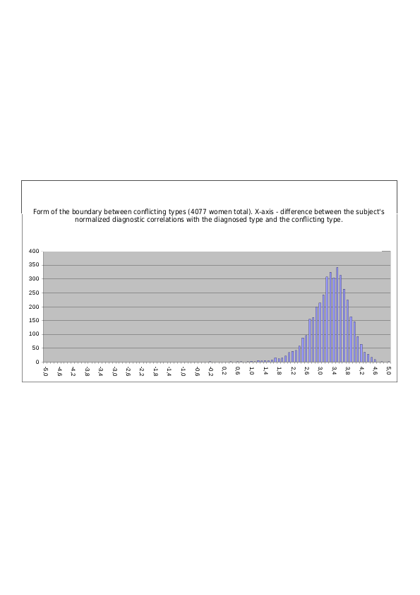
Fig. 7.3. Population distribution of the difference between normalized diagnostic correlations (normalization by Method No. 1) between the type diagnosed in subjects (the “primary type”) and the type in a CONFLICT relation with it (ESI for ILE, ILE for ESI, SEE for LII, LII for SEE, etc.; 16 differences in total for 16 pairs of types). Mixed sample. The density of subjects located exactly on the boundary between the types (the case in which the difference between diagnostic correlations =0) is 0%. The transition from one type to the other is discrete; the boundary is empty, and no accentuated representatives of the population whatsoever are present directly on it.
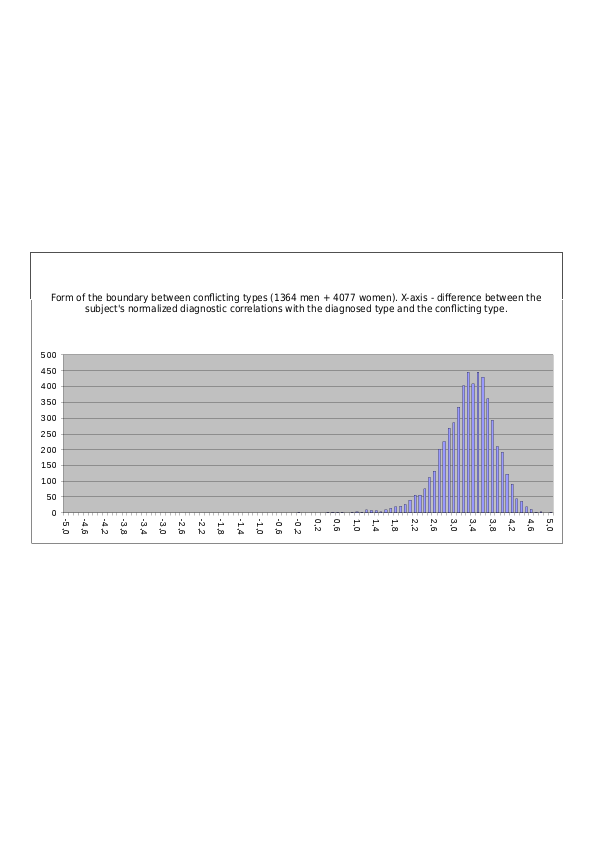
Fig. 7.4. Population distribution of the difference between normalized diagnostic correlations (normalization by Method No. 1) between the type diagnosed in subjects (the “primary type”) and the type in a Conflict relation with it, plus conversely between the conflict type and the subject’s primary type (the diagram combines 32 possible differences in total for 16 pairs of types). Mixed sample. The density of subjects located exactly on the boundary between the types (the case in which the difference between diagnostic correlations =0) is 0%. The boundary becomes “depopulated” already quite far from the point of equality of the correlations. The transition from one type to the other is discrete; the boundary is empty, and no accentuated representatives of the population whatsoever are present directly on it. This does not, however, mean that accentuations superimposed on the primary type in the direction of the conflict type are impossible – the same diagrams show that such accentuations exist, but they fall far short of the immediate boundary with the zone of influence of the conflict type.
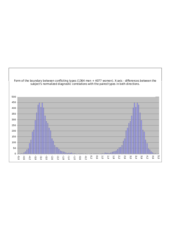
Boundaries Between Types in CONFLICT Relations, with Diagnostic Correlations Normalized by Method No. 2
Fig. 7.5. Population distribution of the difference between normalized diagnostic correlations (normalization by Method No. 2) between the type diagnosed in subjects (the “primary type”) and the type in a CONFLICT relation with it (ESI for ILE, ILE for ESI, SEE for LII, LII for SEE, etc.; 16 differences in total for 16 pairs of types). Mixed sample. The density of subjects located exactly on the boundary between the types (the case in which the difference between diagnostic correlations =0) is 0%. The transition from one type to the other is discrete; the boundary is empty, and no accentuated representatives of the population whatsoever are present directly on it.
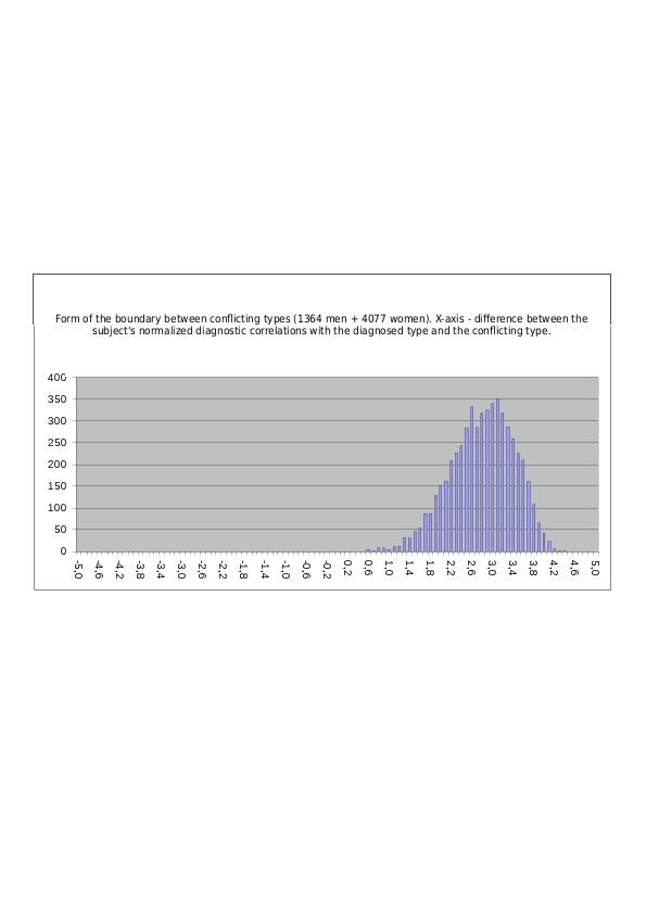
Fig. 7.6. Population distribution of the difference between normalized diagnostic correlations (normalization by Method No. 2) between the type diagnosed in subjects (the “primary type”) and the type in a Conflict relation with it, plus conversely between the conflict type and the subject’s primary type (the diagram combines 32 possible differences in total for 16 pairs of types). Mixed sample. The density of subjects located exactly on the boundary between the types (the case in which the difference between diagnostic correlations =0) is 0%. The boundary becomes “depopulated” already quite far from the point of equality of the correlations. The transition from one type to the other is discrete; the boundary is empty, and no accentuated representatives of the population whatsoever are present directly on it. This does not, however, mean that accentuations superimposed on the primary type in the direction of the conflict type are impossible – the same diagrams show that such accentuations exist, but they fall far short of the immediate boundary with the zone of influence of the conflict type.
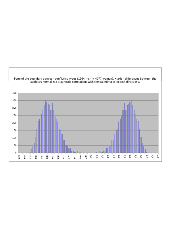
Table 3. Summary table characterizing the boundaries between psychotypes in the metric of normalized diagnostic correlations
| Pair of types | Population mean of the difference between normalized diagnostic correlations, Method No. 1 | Population mean of the difference between normalized diagnostic correlations, Method No. 2 | Half-width (SD) of the population distribution of the difference between normalized diagnostic correlations, Method No. 1 | Half-width (SD) of the population distribution of the difference between normalized diagnostic correlations, Method No. 2 | Ratio of the density of people whose accentuation places them on the two-sided boundary between types to the density of people located “in the core” of a type, Method No. 1 | Ratio of the density of people whose accentuation places them on the two-sided boundary between types to the density of people located “in the core” of a type, Method No. 2 |
|---|---|---|---|---|---|---|
| primary type and “quasi-identical” type (ILE-LIE, etc.) | 0,738 | 0,701 | 0,666 | 0,454 | 0,66 | 0,58 |
| primary type and “kindred” type (ILE-IEE, etc.) | 1,104 | 1,025 | 0,717 | 0,553 | 0,63 | 0,56 |
| primary type and type connected by Business relations (ILE-SLE, etc.) | 1,254 | 1,131 | 0,764 | 0,597 | 0,52 | 0,44 |
| primary type and complete-opposition type (ILE-ILI, etc.) | 1,253 | 1,152 | 0,763 | 0,576 | 0,43 | 0,29 |
| primary type and “mirror” type (ILE-LII, etc.) | 1,607 | 1,358 | 0,678 | 0,570 | 0,14 | 0,13 |
| primary type and “conflict” type (ILE-ESI, etc.) | 3,290 | 2,804 | 0,549 | 0,617 | 0 | 0 |
Results of the Study of Boundaries Between Psychotypes - Provided That the Subjects’ Type Profile Is Composed of the Squares of Diagnostic Correlations with the Signs of the Correlations Retained (That Is, When the Measure of Affinity to a Psychotype Is Not the Correlation but the So-Called “Type Commonality”)
In this case, the subject’s individual type profile is composed not of the quantities R1 - R16 (one diagnostic correlation coefficient for each of the 16 types in the profile), but of the quantities D1 - D16, where D=sign(R)*R*R. If R is the correlation between an individual’s answers and the properties of one of the 16 psychotypes, then D is that proportion of the total variance of the individual’s psychological manifestations (reflected in the specific answers the individual gives to the questionnaire questions) that is attributable to the stable personality characteristics of this standard psychotype. The point is – let us recall from mathematical statistics – that if R is the correlation between the properties of two objects, then R2 is the proportion of their shared common properties within the complete properties of each object. If the numbers R1 – R16 are called diagnostic correlations, then the numbers are called diagnostic type commonalities (or simply type commonalities).
Similarly, for profiles composed of D, we must consider two cases – when we normalize the initial empirical profiles D1 – D16 by the first or the second method. To normalize type commonalities by the second method (using the least-squares method), we require a table analogous to Table 1, representing 16 reference profiles of the 16 psychotypes, but constructed not for R, but for the type commonalities D, likewise averaged over all representatives of each psychotype. The corresponding averaging results (which are also the reference profiles of the 16 psychotypes, expressed as D values normalized by the first method) are presented in Table 4.
Recall that for normalization by the second method, the entire individual type profile of a subject whose primary psychotype has been identified is multiplied by a certain coefficient selected so as to minimize the sum of squared differences between the members of this individual profile and the corresponding members (see Table 4) of the standard profile of the psychotype diagnosed in the subject (that is, the psychotype to which the subject proves closest).
Table 4. Standard TIM profiles for all 16 psychotypes obtained by analyzing the sample of 5441 people. Each profile is located in a row, consists of 16 numbers proportional to the proportion of properties shared by the given psychotype with the properties of other psychotypes and simultaneously proportional to the squares of the correlations with the properties of these psychotypes (“type commonalities”), and reflects the weighted loadings of all 16 different psychotypes by the properties of the “principal” psychotype of the row, marked in yellow.
| ILE | LII | SEI | ESE | SLE | LSI | IEI | EIE | SEE | ESI | ILI | LIE | IEE | EII | SLI | LSE | standard deviation of all profile coefficients in the row | |
|---|---|---|---|---|---|---|---|---|---|---|---|---|---|---|---|---|---|
| ILE | 2,85199 | 0,16093 | -1,0703 | -0,3806 | 0,36832 | -0,4991 | -0,2159 | 0,17226 | -0,1741 | -1,7975 | 0,35815 | 1,05709 | 0,50511 | -0,4991 | -0,2841 | 0,17226 | 1,00000 |
| LII | 0,16093 | 2,85199 | -0,3806 | -1,0703 | -0,4991 | 0,50511 | 0,17226 | -0,2841 | -1,7975 | -0,1741 | 1,05709 | 0,35815 | -0,4991 | 0,36832 | 0,17226 | -0,2159 | 1,00000 |
| SEI | -1,0703 | -0,3806 | 2,85199 | 0,16093 | -0,2159 | 0,17226 | 0,36832 | -0,4991 | 0,35815 | 1,05709 | -0,1741 | -1,7975 | -0,2841 | 0,17226 | 0,50511 | -0,4991 | 1,00000 |
| ESE | -0,3806 | -1,0703 | 0,16093 | 2,85199 | 0,17226 | -0,2841 | -0,4991 | 0,50511 | 1,05709 | 0,35815 | -1,7975 | -0,1741 | 0,17226 | -0,2159 | -0,4991 | 0,36832 | 1,00000 |
| SLE | 0,36832 | -0,4991 | -0,2159 | 0,17226 | 2,85199 | 0,16093 | -1,0703 | -0,3806 | 0,50511 | -0,4991 | -0,2841 | 0,17226 | -0,1741 | -1,7975 | 0,35815 | 1,05709 | 1,00000 |
| LSI | -0,4991 | 0,50511 | 0,17226 | -0,2841 | 0,16093 | 2,85199 | -0,3806 | -1,0703 | -0,4991 | 0,36832 | 0,17226 | -0,2159 | -1,7975 | -0,1741 | 1,05709 | 0,35815 | 1,00000 |
| IEI | -0,2159 | 0,17226 | 0,36832 | -0,4991 | -1,0703 | -0,3806 | 2,85199 | 0,16093 | -0,2841 | 0,17226 | 0,50511 | -0,4991 | 0,35815 | 1,05709 | -0,1741 | -1,7975 | 1,00000 |
| EIE | 0,17226 | -0,2841 | -0,4991 | 0,50511 | -0,3806 | -1,0703 | 0,16093 | 2,85199 | 0,17226 | -0,2159 | -0,4991 | 0,36832 | 1,05709 | 0,35815 | -1,7975 | -0,1741 | 1,00000 |
| SEE | -0,1741 | -1,7975 | 0,35815 | 1,05709 | 0,50511 | -0,4991 | -0,2841 | 0,17226 | 2,85199 | 0,16093 | -1,0703 | -0,3806 | 0,36832 | -0,4991 | -0,2159 | 0,17226 | 1,00000 |
| ESI | -1,7975 | -0,1741 | 1,05709 | 0,35815 | -0,4991 | 0,36832 | 0,17226 | -0,2159 | 0,16093 | 2,85199 | -0,3806 | -1,0703 | -0,4991 | 0,50511 | 0,17226 | -0,2841 | 1,00000 |
| ILI | 0,35815 | 1,05709 | -0,1741 | -1,7975 | -0,2841 | 0,17226 | 0,50511 | -0,4991 | -1,0703 | -0,3806 | 2,85199 | 0,16093 | -0,2159 | 0,17226 | 0,36832 | -0,4991 | 1,00000 |
| LIE | 1,05709 | 0,35815 | -1,7975 | -0,1741 | 0,17226 | -0,2159 | -0,4991 | 0,36832 | -0,3806 | -1,0703 | 0,16093 | 2,85199 | 0,17226 | -0,2841 | -0,4991 | 0,50511 | 1,00000 |
| IEE | 0,50511 | -0,4991 | -0,2841 | 0,17226 | -0,1741 | -1,7975 | 0,35815 | 1,05709 | 0,36832 | -0,4991 | -0,2159 | 0,17226 | 2,85199 | 0,16093 | -1,0703 | -0,3806 | 1,00000 |
| EII | -0,4991 | 0,36832 | 0,17226 | -0,2159 | -1,7975 | -0,1741 | 1,05709 | 0,35815 | -0,4991 | 0,50511 | 0,17226 | -0,2841 | 0,16093 | 2,85199 | -0,3806 | -1,0703 | 1,00000 |
| SLI | -0,2841 | 0,17226 | 0,50511 | -0,4991 | 0,35815 | 1,05709 | -0,1741 | -1,7975 | -0,2159 | 0,17226 | 0,36832 | -0,4991 | -1,0703 | -0,3806 | 2,85199 | 0,16093 | 1,00000 |
| LSE | 0,17226 | -0,2159 | -0,4991 | 0,36832 | 1,05709 | 0,35815 | -1,7975 | -0,1741 | 0,17226 | -0,2841 | -0,4991 | 0,50511 | -0,3806 | -1,0703 | 0,16093 | 2,85199 | 1,00000 |
Boundaries Between QUASI-IDENTICAL Types - with Empirical Type-Commonality Profiles D1-D16 Normalized by Method No. 1
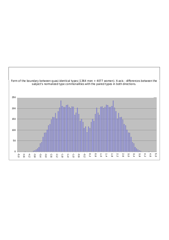
Fig. 8.1. Population distribution of the difference between normalized type commonalities (normalization by Method No. 1) between the type diagnosed in subjects (the “primary type”) and its quasi-identical type (ILI for LII, LII for ILI, LSE for SLE, SLE for LSE, etc.; 16 possible differences in total for 16 pairs of types). Mixed sample. The relative density of subjects located exactly on the boundary between the types (the case in which the difference between type commonalities =0) is 19% of the maximum density (=45/235*100%). The transition from one type to the other is therefore smooth and continuous, although the boundary between the types is nevertheless visible in the decline in the probability density of finding subjects on it.
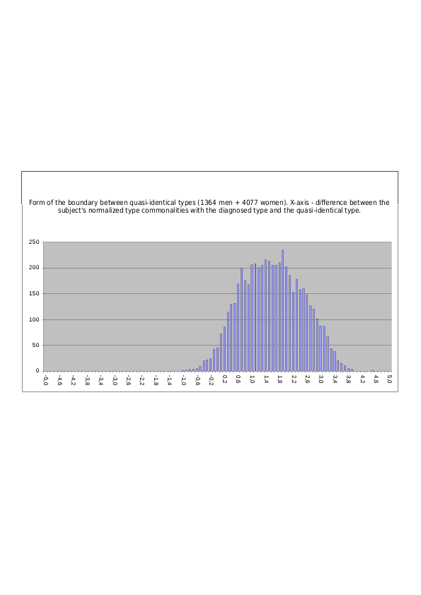
Fig. 8.2. Population distribution of the difference between normalized type commonalities (normalization by Method No. 1) between the type diagnosed in subjects (the “primary type”) and its quasi-identical type, plus between the quasi-identical and primary types (yielding 32 possible differences in total for 16 pairs of types). Mixed sample. The relative density of subjects located exactly on the boundary between the types (the case in which the difference between type commonalities =0) is approximately 38% (90/235*100%) of the maximum density found at the center of each psychotype in the pair. Compared with the preceding figure, the relative boundary density has doubled because here the possibility that the subject belongs to either one or the other type in the pair is taken into account – as a result, the absolute density at the boundary between them doubles, while the probability of finding a subject at the center of each peak does not increase because it is summed with the flank of the other peak, which declines to zero. The transition from one type to the other is theoretically smooth and continuous, although the boundary between the types is nevertheless clearly visible in the decline in the probability density of finding subjects on it.
Boundaries Between QUASI-IDENTICAL Types with Type Commonalities Normalized by Method No. 2
Fig. 8.3. Population distribution of the difference between normalized type commonalities (normalization by Method No. 2) between the type diagnosed in subjects (the “primary type”) and its quasi-identical type (ILI for LII, LII for ILI, LSE for SLE, SLE for LSE, etc.; 16 possible differences in total for 16 pairs of types). Mixed sample. The relative density of subjects located exactly on the boundary between the types (the case in which the difference between type commonalities =0) is 22% of the maximum density (=56/252*100%). The transition from one type to the other is therefore smooth and continuous, although the boundary between the types is nevertheless visible in the decline in the probability density of finding subjects on it.
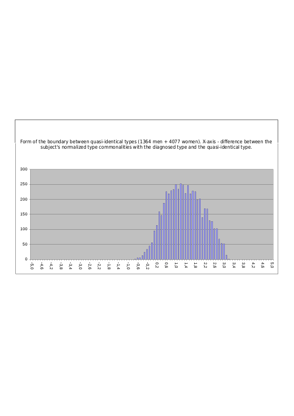
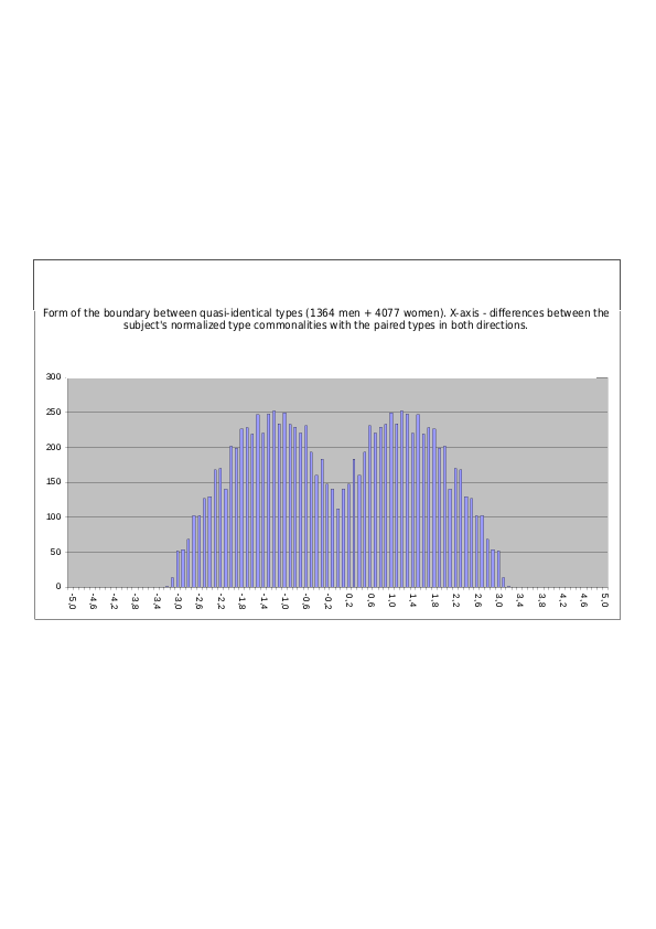
Fig. 8.4. Population distribution of the difference between normalized type commonalities (normalization by Method No. 2) between the type diagnosed in subjects (the “primary type”) and its quasi-identical type, plus between the quasi-identical and primary types (yielding 32 possible differences in total for 16 pairs of types). Mixed sample. The relative density of subjects located exactly on the boundary between the types (the case in which the difference between type commonalities =0) is approximately 44% (112/252*100%) of the maximum density found at the center of each psychotype in the pair. Compared with the preceding figure, the relative boundary density has doubled because here the possibility that the subject belongs to either one or the other type in the pair is taken into account – as a result, the absolute density at the boundary between them doubles, while the probability of finding a subject at the center of each peak does not increase because it is summed with the flank of the other peak, which declines to zero. The transition from one type to the other is theoretically smooth and continuous, although the boundary between the types is nevertheless clearly visible in the decline in the probability density of finding subjects on it.
Boundaries Between KINDRED Types with Type Commonalities Normalized by Method No. 1
Fig. 9.1. Population distribution of the difference between normalized type commonalities (normalization by Method No. 1) between the type diagnosed in subjects (the “primary type”) and its kindred type (IEE for ILE, ILE for IEE, LSI for LII, LII for LSI, etc.; 16 possible differences in total for 16 pairs of types). Mixed sample. The relative density of subjects located exactly on the boundary between the types (the case in which the difference between type commonalities =0) is 11% of the maximum density (=32/298*100%). The transition from one type to the other is smooth and continuous, although the boundary between the types is nevertheless clearly visible in the decline in the probability density of finding subjects on it.
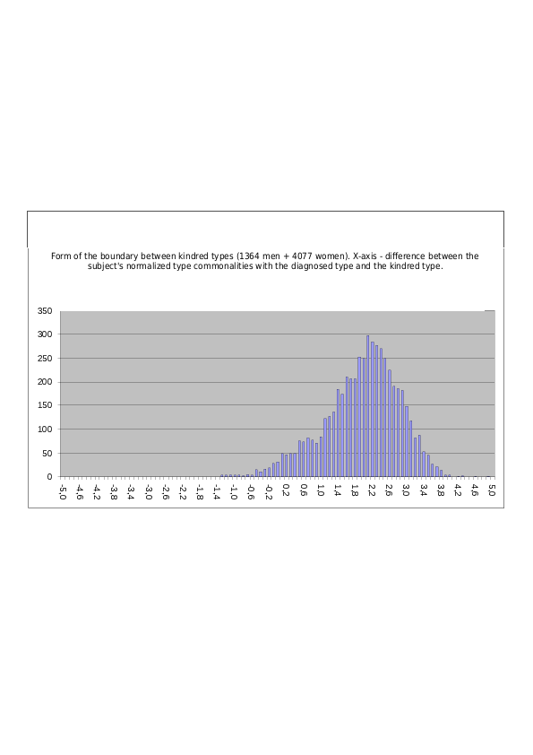
Fig. 9.2. Population distribution of the difference between normalized type commonalities (normalization by Method No. 1) between the type diagnosed in subjects (the “primary type”) and its kindred type, plus between the kindred and primary types (the diagram combines 32 differences in total for 16 pairs of types). Mixed sample. The relative density of subjects located exactly on the boundary between the types (the case in which the difference between type commonalities =0) is approximately 21% (=64/298*100%) of the maximum density found at the center of each psychotype in the pair. Compared with the preceding figure, the boundary density has doubled because here the possibility that the subject belongs to either one or the other type in the pair is taken into account – as a result, the density at the boundary between them doubles. The transition from one type to the other is continuous, although the boundary between the types is nevertheless clearly visible from the sharp decline in the probability density of finding subjects on it.
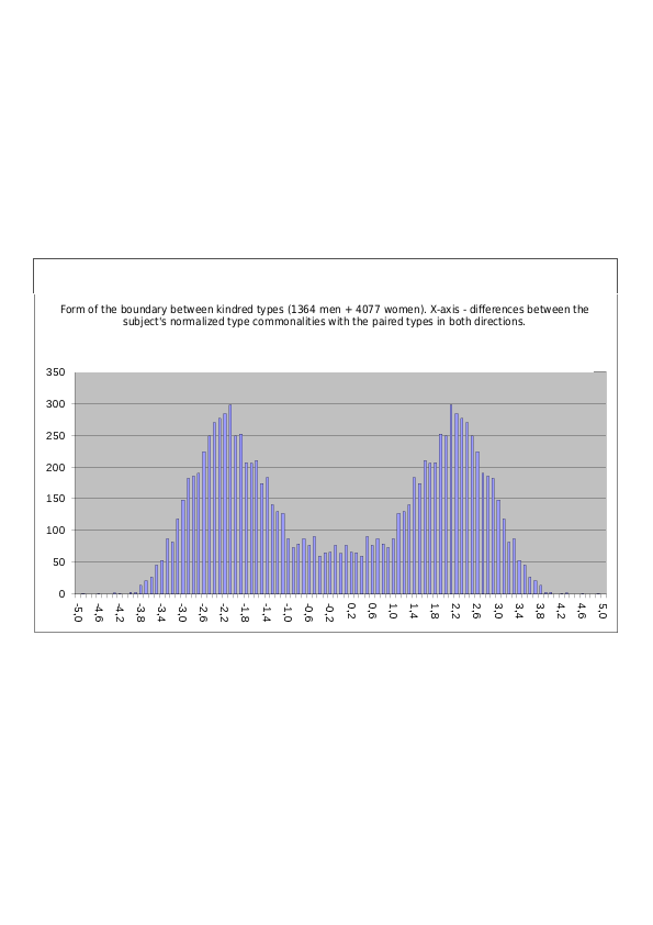
Boundaries Between KINDRED Types with Type Commonalities Normalized by Method No. 2
Fig. 9.3. Population distribution of the difference between normalized type commonalities (normalization by Method No. 2) between the type diagnosed in subjects (the “primary type”) and its kindred type (IEE for ILE, ILE for IEE, LSI for LII, LII for LSI, etc.; 16 possible differences in total for 16 pairs of types). Mixed sample. The relative density of subjects located exactly on the boundary between the types (the case in which the difference between type commonalities =0) is approximately 18% of the maximum density (=50/280*100%). The transition from one type to the other is smooth and continuous, although the boundary between the types is nevertheless clearly visible in the decline in the probability density of finding subjects on it.
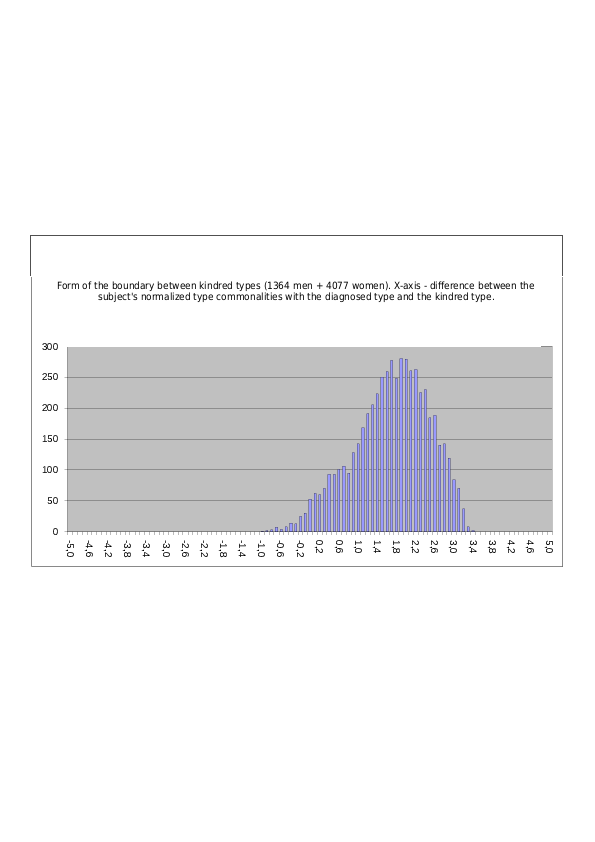
Fig. 9.4. Population distribution of the difference between normalized type commonalities (normalization by Method No. 2) between the type diagnosed in subjects (the “primary type”) and its kindred type, plus between the kindred and primary types (the diagram combines 32 differences in total for 16 pairs of types). Mixed sample. The relative density of subjects located exactly on the boundary between the types (the case in which the difference between type commonalities =0) is approximately 36% (=100/280*100%) of the maximum density found at the center of each psychotype in the pair. Compared with the preceding figure, the boundary density has doubled because here the possibility that the subject belongs to either one or the other type in the pair is taken into account – as a result, the density at the boundary between them doubles. The transition from one type to the other is smooth and continuous, although the boundary between the types is nevertheless clearly visible in the decline in the probability density of finding subjects on it.
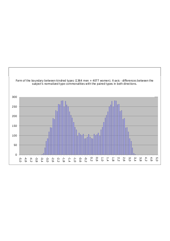
Boundaries Between Types in BUSINESS RELATIONS with Type Commonalities Normalized by Method No. 1
Fig. 10.1. Population distribution of the difference between normalized type commonalities (normalization by Method No. 1) between the type diagnosed in subjects (the “primary type”) and the type in a Business relation with it (SLE for ILE, ILE for SLE, EII for LII, LII for EII, etc.; 16 possible differences in total for 16 pairs of types). Mixed sample. The relative density of subjects located exactly on the boundary between the types (the case in which the difference between type commonalities =0) is approximately 9% of the maximum density (=28/301*100%). The transition from one type to the other remains formally continuous, although the boundary between the types is nevertheless clearly visible from the sharp decline in the probability density of finding subjects on it.
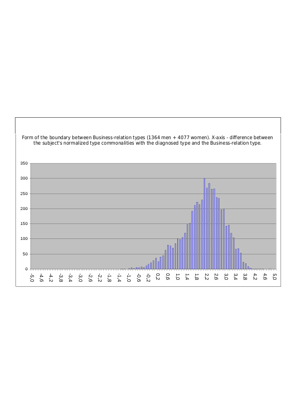
Fig. 10.2. Population distribution of the difference between normalized type commonalities (normalization by Method No. 1) between the type diagnosed in subjects (the “primary type”) and the type in a Business relation with it, plus between the Business-related and primary types (the diagram combines 32 differences in total for 16 pairs of types). Mixed sample. The relative density of subjects located exactly on the boundary between the types (the case in which the difference between type commonalities =0) is approximately 19% (=56/301*100%) of the maximum density found at the center of each psychotype in the pair. Compared with the preceding figure, the boundary density has doubled because here the possibility that the subject belongs to either one or the other type in the pair is taken into account – as a result, the density at the boundary between them doubles. The transition from one type to the other remains formally continuous, although the boundary between the types is nevertheless clearly visible from the sharp decline in the probability density of finding subjects on it.
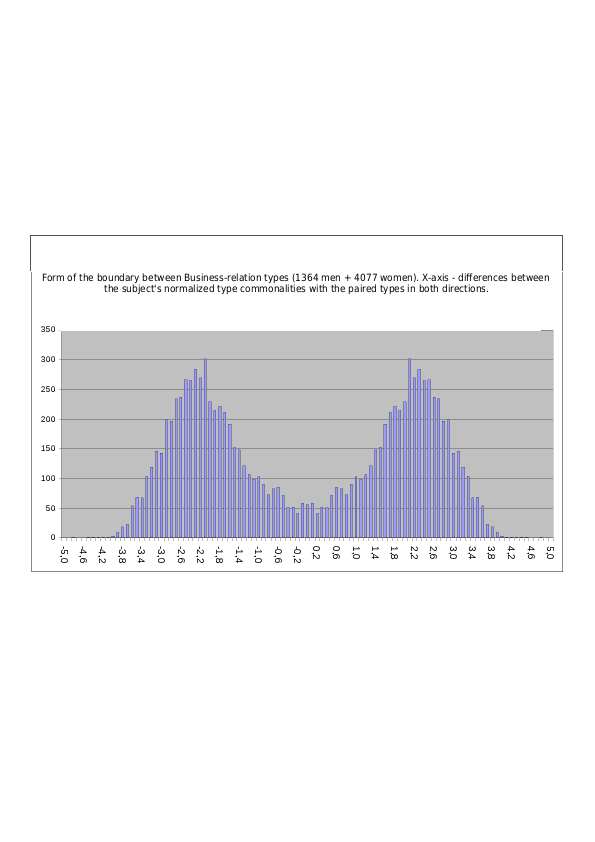
Boundaries Between Types in BUSINESS RELATIONS with Type Commonalities Normalized by Method No. 2
Fig. 10.3. Population distribution of the difference between normalized type commonalities (normalization by Method No. 2) between the type diagnosed in subjects (the “primary type”) and the type in a Business relation with it (SLE for ILE, ILE for SLE, EII for LII, LII for EII, etc.; 16 possible differences in total for 16 pairs of types). Mixed sample. The relative density of subjects located exactly on the boundary between the types (the case in which the difference between type commonalities =0) is approximately 14% of the maximum density (=41/289*100%). The transition from one type to the other remains formally continuous, although the boundary between the types is nevertheless clearly visible from the sharp decline in the probability density of finding subjects on it.
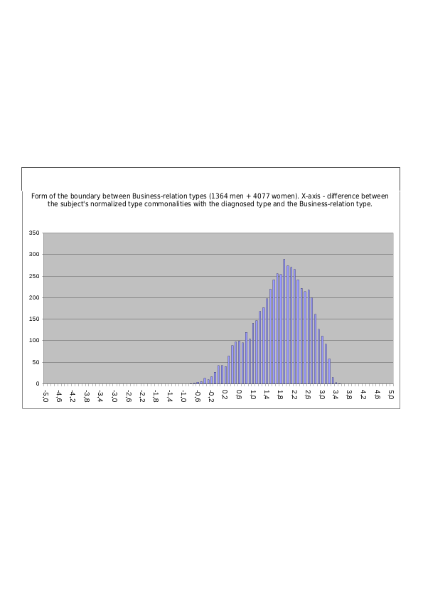
Fig. 10.4. Population distribution of the difference between normalized type commonalities (normalization by Method No. 2) between the type diagnosed in subjects (the “primary type”) and the type in a Business relation with it, plus between the Business-related and primary types (the diagram combines 32 differences in total for 16 pairs of types). Mixed sample. The relative density of subjects located exactly on the boundary between the types (the case in which the difference between type commonalities =0) is approximately 28% (=82/289*100%) of the maximum density found at the center of each psychotype in the pair. Compared with the preceding figure, the boundary density has doubled because here the possibility that the subject belongs to either one or the other type in the pair is taken into account – as a result, the density at the boundary between them doubles. The transition from one type to the other remains formally continuous, although the boundary between the types is nevertheless clearly visible from the sharp decline in the probability density of finding subjects on it.
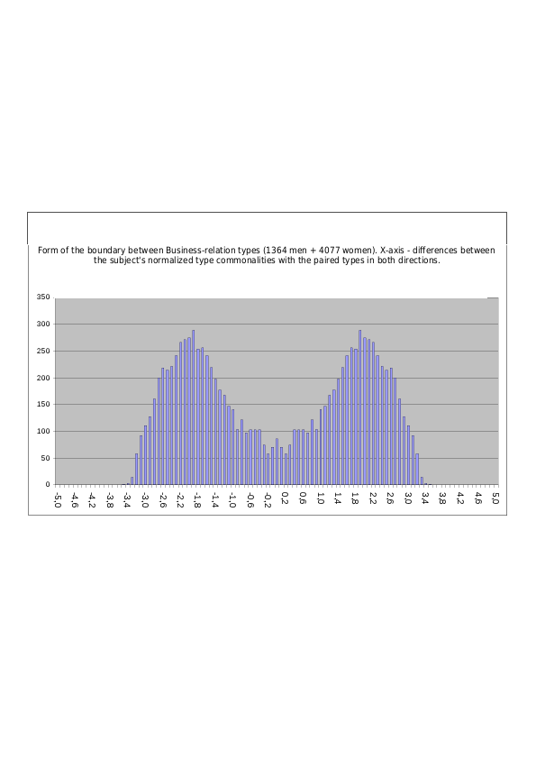
Boundaries Between Types in COMPLETE OPPOSITION Relations, with Type Commonalities Normalized by Method No. 1
Fig. 11.1. Population distribution of the difference between normalized type commonalities (normalization by Method No. 1) between the type diagnosed in subjects (the “primary type”) and the type in a complete opposition relation with it (ILI for ILE, ILE for ILI, LIE for LII, LII for LIE, etc.; 16 possible differences in total for 16 pairs of types). Mixed sample. The relative density of subjects located exactly on the boundary between the types (the case in which the difference between type commonalities =0) is approximately 6% (=19/307*100%) of the maximum density found at the center of the psychotype. The transition from one type to the other remains smooth and continuous; the boundary is not empty, and individual accentuated cases from the population are present on it, although the boundary between the types is nevertheless clearly visible from the sharp decline in the probability density of finding subjects on it.
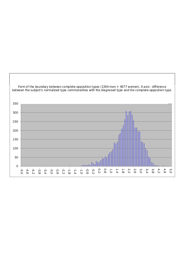
Fig. 11.2. Population distribution of the difference between normalized type commonalities (normalization by Method No. 1) between the type diagnosed in subjects (the “primary type”) and the type in a complete opposition relation with it, plus between the type in a complete opposition relation and the primary type (the diagram combines 32 possible differences in total for 16 pairs of types). Mixed sample. The relative density of subjects located exactly on the boundary between the types (the case in which the difference between type commonalities =0) is approximately 12% (=38/307*100%) of the maximum density found at the center of each psychotype in the pair. Compared with the preceding figure, the boundary density has doubled because here the possibility that the subject belongs to either one or the other type in the pair is taken into account – as a result, the density at the boundary between them doubles. The transition from one type to the other remains formally continuous; the boundary is not empty, and individual sharply accentuated cases from the population are present on it, although the boundary between the types is nevertheless clearly visible from the sharp decline in the probability density of finding subjects on it.
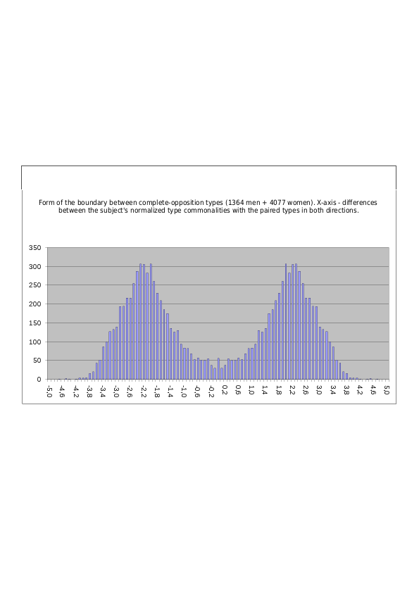
Boundaries Between Types in COMPLETE OPPOSITION Relations, with Type Commonalities Normalized by Method No. 2
Fig. 11.3. Population distribution of the difference between normalized type commonalities (normalization by Method No. 2) between the type diagnosed in subjects (the “primary type”) and the type in a complete opposition relation with it (ILI for ILE, ILE for ILI, LIE for LII, LII for LIE, etc.; 16 possible differences in total for 16 pairs of types). Mixed sample. The relative density of subjects located exactly on the boundary between the types (the case in which the difference between type commonalities =0) is approximately 10% (=30/303*100%) of the maximum density found at the center of the psychotype. The transition from one type to the other remains smooth and continuous; the boundary is not empty, and individual accentuated cases from the population are present on it, although the boundary between the types is nevertheless clearly visible from the sharp decline in the probability density of finding subjects on it.
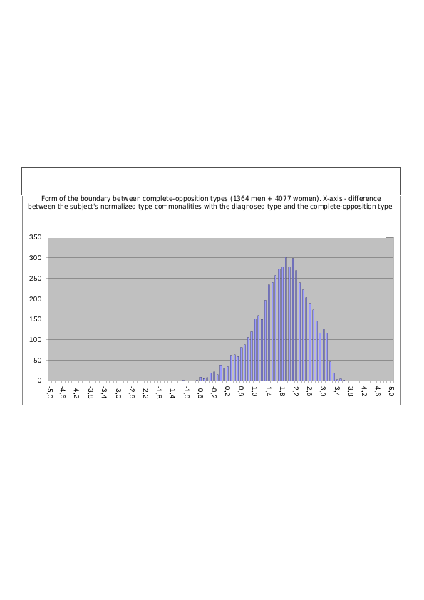
Fig. 11.4. Population distribution of the difference between normalized type commonalities (normalization by Method No. 2) between the type diagnosed in subjects (the “primary type”) and the type in a complete opposition relation with it, plus between the type in a complete opposition relation and the primary type (the diagram combines 32 possible differences in total for 16 pairs of types). Mixed sample. The relative density of subjects located exactly on the boundary between the types (the case in which the difference between type commonalities =0) is approximately 20% (=60/303*100%) of the maximum density found at the center of each psychotype in the pair. Compared with the preceding figure, the boundary density has doubled because here the possibility that the subject belongs to either one or the other type in the pair is taken into account – as a result, the density at the boundary between them doubles. The transition from one type to the other remains formally continuous; the boundary is not empty, and individual sharply accentuated cases from the population are present on it, although the boundary between the types is nevertheless clearly visible from the sharp decline in the probability density of finding subjects on it.
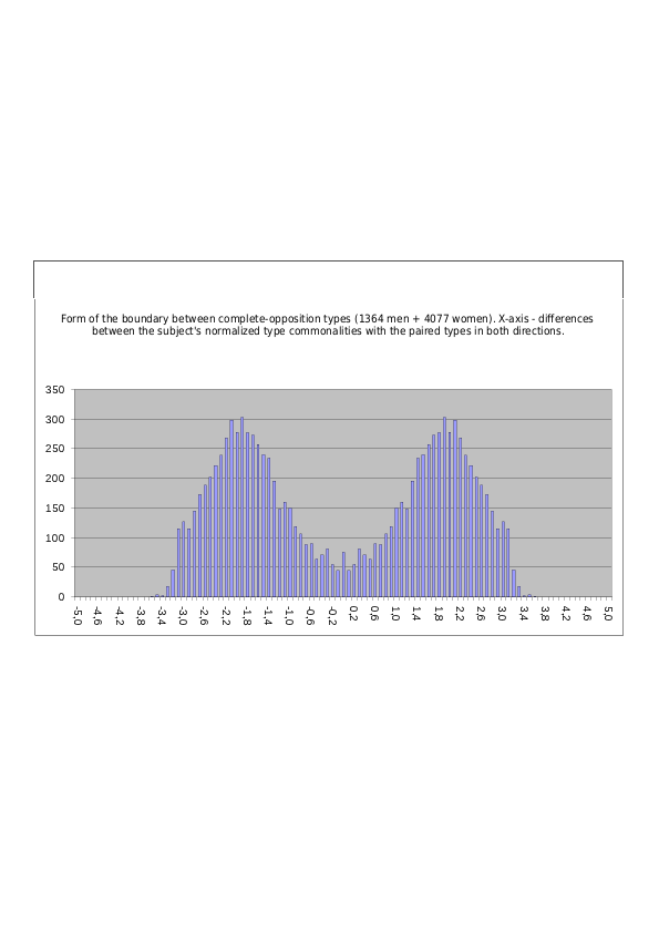
Boundaries Between Types in MIRROR Relations, with Type Commonalities Normalized by Method No. 1
Fig. 12.1. Population distribution of the difference between normalized type commonalities (normalization by Method No. 1) between the type diagnosed in subjects (the “primary type”) and the type in a Mirror relation with it (LII for ILE, ILE for LII, ESE for SEI, SEI for ESE, etc.; 16 possible differences in total for 16 pairs of types). Mixed sample. The relative density of subjects located exactly on the boundary between the types (the case in which the difference between type commonalities =0) is approximately 2% (=7/341*100%) of the maximum density found at the center of the psychotype. The transition from one type to the other remains smooth and continuous; the boundary is not empty, and individual accentuated cases from the population are present on it, although the boundary between the types is nevertheless clearly visible from the sharp decline in the probability density of finding subjects on it.
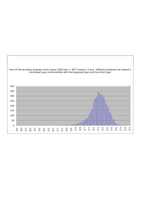
Fig. 12.2. Population distribution of the difference between normalized type commonalities (normalization by Method No. 1) between the type diagnosed in subjects (the “primary type”) and the type in a Mirror relation with it, plus conversely between the mirror type and the subject’s primary type (the diagram combines 32 possible differences in total for 16 pairs of types). Mixed sample. The relative density of subjects located exactly on the boundary between the types (the case in which the difference between type commonalities =0) is approximately 4% (14/341*100%) of the maximum density found at the center of each psychotype in the pair. Compared with the preceding figure, the boundary density has doubled because here the possibility that the subject belongs to either one or the other type in the pair is taken into account – as a result, the density at the boundary between them doubles. In a purely formal sense, the transition from one type to the other remains continuous; the boundary is not empty, and individual sharply accentuated cases from the population are present on it, although the boundary between the types is nevertheless clearly visible from the very sharp, nearly to zero, decline in the probability density of finding subjects on it.
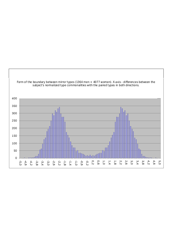
Boundaries Between Types in MIRROR Relations, with Type Commonalities Normalized by Method No. 2
Fig. 12.3. Population distribution of the difference between normalized type commonalities (normalization by Method No. 2) between the type diagnosed in subjects (the “primary type”) and the type in a Mirror relation with it (LII for ILE, ILE for LII, ESE for SEI, SEI for ESE, etc.; 16 possible differences in total for 16 pairs of types). Mixed sample. The relative density of subjects located exactly on the boundary between the types (the case in which the difference between type commonalities =0) is approximately 5% (=15/327*100%) of the maximum density found at the center of the psychotype. The transition from one type to the other remains smooth and continuous; the boundary is not empty, and individual accentuated cases from the population are present on it, although the boundary between the types is nevertheless clearly visible from the sharp decline in the probability density of finding subjects on it.
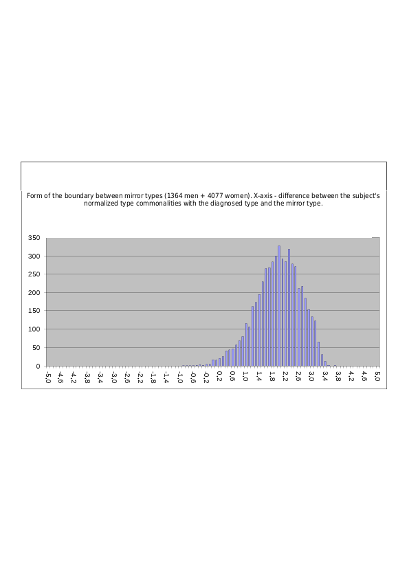
Fig. 12.4. Population distribution of the difference between normalized type commonalities (normalization by Method No. 2) between the type diagnosed in subjects (the “primary type”) and the type in a Mirror relation with it, plus conversely between the mirror type and the subject’s primary type (the diagram combines 32 possible differences in total for 16 pairs of types). Mixed sample. The relative density of subjects located exactly on the boundary between the types (the case in which the difference between type commonalities =0) is approximately 9% (30/327*100%) of the maximum density found at the center of each psychotype in the pair. Compared with the preceding figure, the boundary density has doubled because here the possibility that the subject belongs to either one or the other type in the pair is taken into account – as a result, the density at the boundary between them doubles. In a purely formal sense, the transition from one type to the other remains continuous; the boundary is not empty, and individual sharply accentuated cases from the population are present on it, although the boundary between the types is nevertheless clearly visible from the very sharp, nearly to zero, decline in the probability density of finding subjects on it.
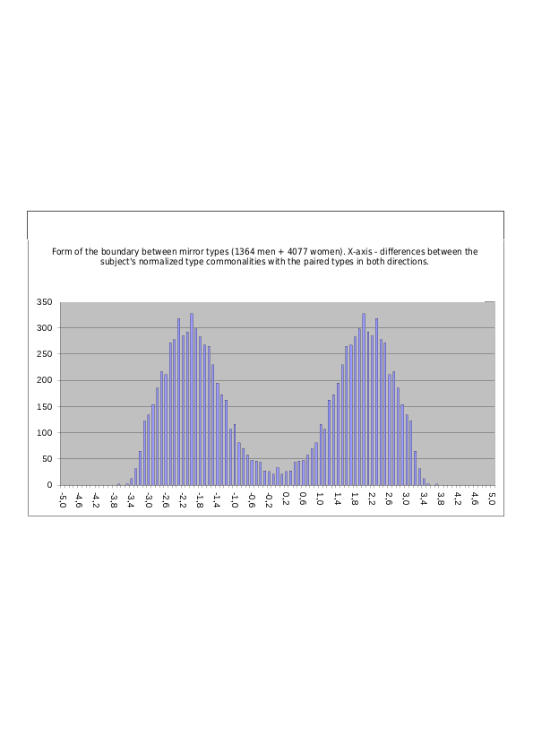
Boundaries Between Types in CONFLICT Relations, with Type Commonalities Normalized by Method No. 1
Fig. 13.1. Population distribution of the difference between normalized type commonalities (normalization by Method No. 1) between the type diagnosed in subjects (the “primary type”) and the type in a CONFLICT relation with it (ESI for ILE, ILE for ESI, SEE for LII, LII for SEE, etc.; 16 differences in total for 16 pairs of types). Mixed sample. The density of subjects located exactly on the boundary between the types (the case in which the difference between type commonalities =0) is 0%. The transition from one type to the other is discrete; the boundary is empty, and no accentuated representatives of the population whatsoever are present directly on it.
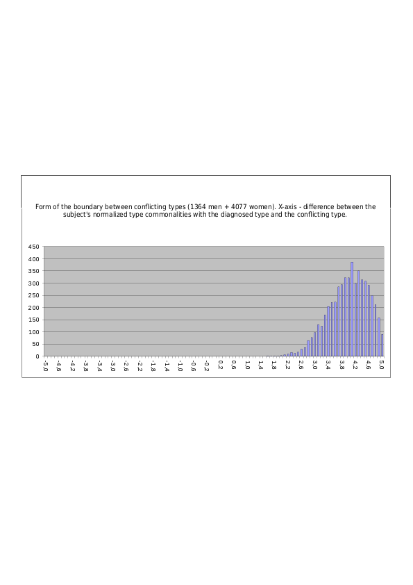
Fig. 13.2. Population distribution of the difference between normalized type commonalities (normalization by Method No. 1) between the type diagnosed in subjects (the “primary type”) and the type in a Conflict relation with it, plus conversely between the conflict type and the subject’s primary type (the diagram combines 32 possible differences in total for 16 pairs of types). Mixed sample. The density of subjects located exactly on the boundary between the types (the case in which the difference between type commonalities =0) is 0%. The boundary becomes “depopulated” already quite far from the point of equality of the correlations. The transition from one type to the other is discrete; the boundary is empty, and no accentuated representatives of the population whatsoever are present directly on it. This does not, however, mean that accentuations superimposed on the primary type in the direction of the conflict type are impossible – the same diagrams show that such accentuations exist, but they fall far short of the immediate boundary with the zone of influence of the conflict type.
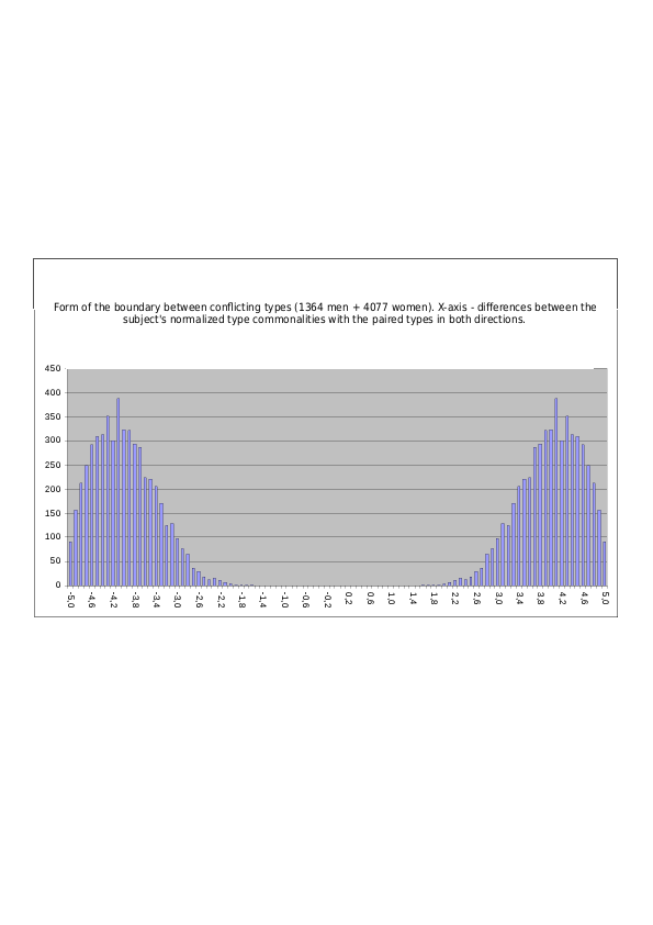
Boundaries Between Types in CONFLICT Relations, with Type Commonalities Normalized by Method No. 2
Fig. 13.3. Population distribution of the difference between normalized type commonalities (normalization by Method No. 2) between the type diagnosed in subjects (the “primary type”) and the type in a CONFLICT relation with it (ESI for ILE, ILE for ESI, SEE for LII, LII for SEE, etc.; 16 differences in total for 16 pairs of types). Mixed sample. The density of subjects located exactly on the boundary between the types (the case in which the difference between type commonalities =0) is 0%. The transition from one type to the other is discrete; the boundary is empty, and no accentuated representatives of the population whatsoever are present directly on it.
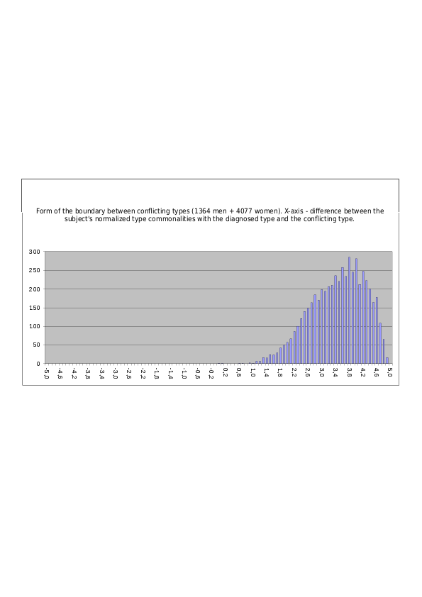
Fig. 13.4. Population distribution of the difference between normalized type commonalities (normalization by Method No. 2) between the type diagnosed in subjects (the “primary type”) and the type in a Conflict relation with it, plus conversely between the conflict type and the subject’s primary type (the diagram combines 32 possible differences in total for 16 pairs of types). Mixed sample. The density of subjects located exactly on the boundary between the types (the case in which the difference between type commonalities =0) is 0%. The boundary becomes “depopulated” already quite far from the point of equality of the correlations. The transition from one type to the other is discrete; the boundary is empty, and no accentuated representatives of the population whatsoever are present directly on it. This does not, however, mean that accentuations superimposed on the primary type in the direction of the conflict type are impossible – the same diagrams show that such accentuations exist, but they fall far short of the immediate boundary with the zone of influence of the conflict type.
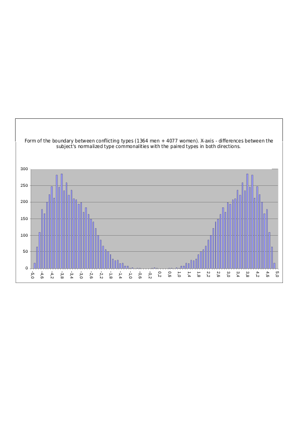
Table 5. Summary table characterizing the boundaries between psychotypes in the metric of normalized type commonalities
| Pair of types | Population mean of the difference between normalized type commonalities, Method No. 1 | Population mean of the difference between normalized type commonalities, Method No. 2 | Half-width (SD) of the population distribution of the difference between normalized type commonalities, Method No. 1 | Half-width (SD) of the population distribution of the difference between normalized type commonalities, Method No. 2 | Ratio of the density of people whose accentuation places them on the two-sided boundary between types to the density of people located “in the core” of a type, Method No. 1 | Ratio of the density of people whose accentuation places them on the two-sided boundary between types to the density of people located “in the core” of a type, Method No. 2 |
|---|---|---|---|---|---|---|
| primary type and “quasi-identical” type (ILE-LIE, etc.) | 1,588 | 1,359 | 0,890 | 0,774 | 0,38 | 0,44 |
| primary type and “kindred” type (ILE-IEE, etc.) | 1,956 | 1,697 | 0,872 | 0,793 | 0,21 | 0,36 |
| primary type and type connected by Business relations (ILE-SLE, etc.) | 2,055 | 1,782 | 0,863 | 0,792 | 0,19 | 0,28 |
| primary type and complete-opposition type (ILE-ILI, etc.) | 2,076 | 1,799 | 0,826 | 0,764 | 0,12 | 0,20 |
| primary type and “mirror” type (ILE-LII, etc.) | 2,271 | 1,963 | 0,720 | 0,691 | 0,04 | 0,09 |
| primary type and “conflict” type (ILE-ESI, etc.) | 4,007 | 3,454 | 0,604 | 0,796 | 0 | 0 |
Part 2 – Boundaries Between the Poles of Socionic Traits
Within the present study, the degree to which subjects quantitatively belonged to extroverts or introverts, to the thinking or emotional-feeling type pole, to statics or dynamics, etc., was calculated not directly, using any special scales for diagnosing extraversion-introversion, logic-ethics, etc., but indirectly, on the basis of the experimentally obtained individual type profiles of the subjects. This was done as follows. Suppose there is a subject’s type profile consisting of 16 type loadings normalized by Method 1 or Method 2 (see Part 1 of the article). These loadings, before normalization, may be either the primary diagnostic correlations, directly measured from the questionnaire, between the subject’s answers and the reference answers of each of the 16 sociotypes, or the variance-based “type commonalities,” equal to the square of the corresponding correlation and taken with the sign of that correlation. To obtain, for example, a quantitative value of a subject’s verticity on the basis of such profiles, we take the mean value of the subject’s loadings for all 8 extroverted types in the profile, then subtract the mean value of the loadings for the 8 introverted types in the profile, and divide the resulting difference by two. The resulting index characterizes the subject’s verticity in the metric of normalized diagnostic correlations or normalized type commonalities, depending on whether the type profile of correlations or of variance-based commonalities was used for the calculation. With this approach, incidentally, it occasionally happens that a person diagnosed as a representative of an extroverted type (for example, LIE) receives, for the balance calculated in this way, not a positive verticity index, as would be appropriate according to the type, but a weakly negative one, which much more often corresponds to introverted types. That is, an LIE or representative of another extroverted type may, in principle, on the sum of all of his or her behavioral manifestations, turn out to be an ambivert with a slight introverted inclination (although only in a very small percentage of cases – in most cases the sign of verticity corresponds to the verticity of the primary diagnosed type). This apparent “mismatch” is associated with the circumstance that the verticity index calculated from the integral type profile takes into account not only the subject’s primary type, but also all of the subject’s objectively present socionic accentuations, which reflect the level of development in the person of absolutely all 8 socionic functions, rather than only the verticity of the program function alone. This is, in fact, an advantage rather than a disadvantage of the method.
The indices of all the other 14 socionic traits are calculated analogously. As a result of summing, with a plus or minus sign, all 16 empirically identified type loadings in such calculations, a quantitative index is obtained for each socionic trait. In most cases its final sign coincides with the polarity of the calculated trait prescribed by the subject’s type, but occasionally it may differ from it. If the sign can “wander” slightly, then the magnitude of the calculated trait can all the more so “wander.” Thus, if a subject is diagnosed as a representative of a logical type, while the logic-ethics balance calculated from the type profile considerably exceeds the mean logic values ordinarily obtained for that type, one may speak of a logical accentuation of this subject additional to the type; if, conversely, the subject’s logic-ethics balance is softened and shifted toward zero, then we speak of an additional ethical-emotional accentuation superimposed on the subject’s basic logical type.
When the magnitude of socionic traits is calculated by the procedure described above, not one diagnostic correlation but 16 such correlations are used at once, that is, the transmission of 16 selectively tuned filters is summed. This greatly blurs the selectivity of the filters’ tuning and brings the method of quantitatively measuring extraversion-introversion and other socionic traits closer to methods based on the use of so-called “continuous scales,” which do not use resonance tuning to isolate local zones of multidimensional psychological space. Therefore, if the study of the population distribution of the magnitudes of socionic traits reveals their bimodality, at least for some of them, this will be a stronger argument in favor of objective boundaries between psychotypes than even the results presented in Part 1 of the present article.
EXTRAVERSION-INTROVERSION
Distribution in the experimental sample of 5441 people of the magnitude of the extraversion-introversion trait calculated from the subjects’ type profiles – when diagnostic correlations are used in the type profile and normalized by Method No. 1:
Fig. 14.1.1. Distribution of verticity magnitude. Positive values correspond to extroverts. Male sample (1364 men)
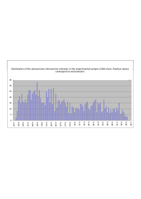
Fig. 14.1.2. Distribution of verticity magnitude. Positive values correspond to extroverts. Female sample (4077 women)
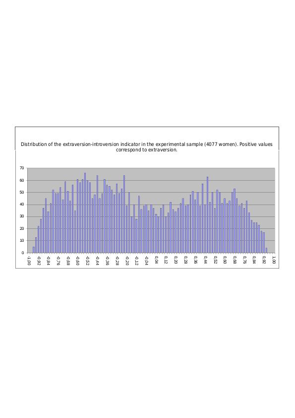
Fig. 14.1.3. Distribution of verticity magnitude. Positive values correspond to extroverts. Mixed sample (1364 men + 4077 women)
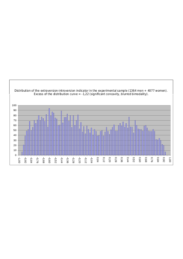
Distribution in the experimental sample of 5441 people of the magnitude of the extraversion-introversion trait calculated from the subjects’ type profiles – when diagnostic correlations are used in the type profile and normalized by Method No. 2:
Fig. 14.2.1. Distribution of verticity magnitude. Positive values correspond to extroverts. Male sample (1364 men)
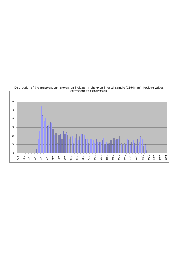
Fig. 14.2.2. Distribution of verticity magnitude. Positive values correspond to extroverts. Female sample (4077 women)
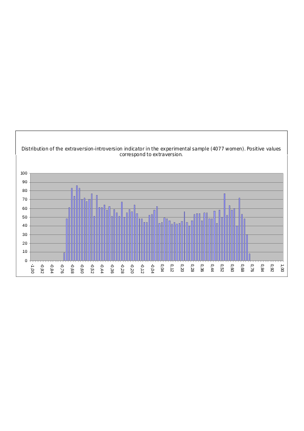
Fig. 14.2.3. Distribution of verticity magnitude. Positive values correspond to extroverts. Mixed sample (1364 men + 4077 women)
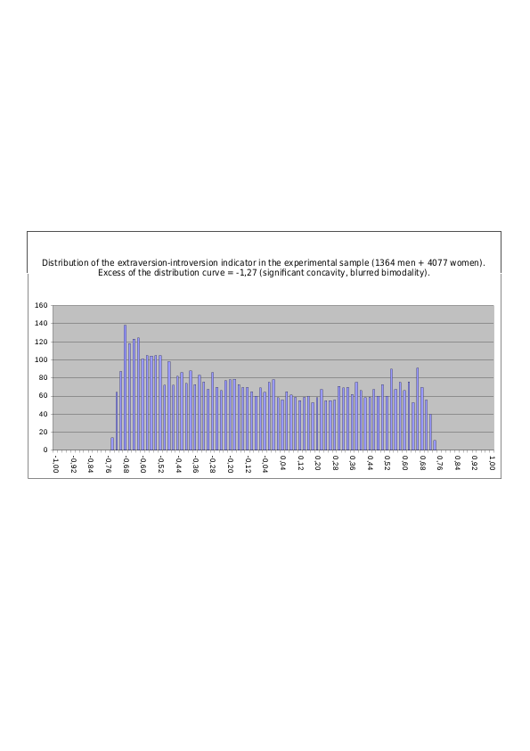
Distribution in the experimental sample of 5441 people of the magnitude of the extraversion-introversion trait calculated from the subjects’ type profiles – when variance-based type commonalities are used in the type profile and normalized by Method No. 1:
Fig. 14.3.1. Distribution of verticity magnitude. Positive values correspond to extroverts. Male sample (1364 men)
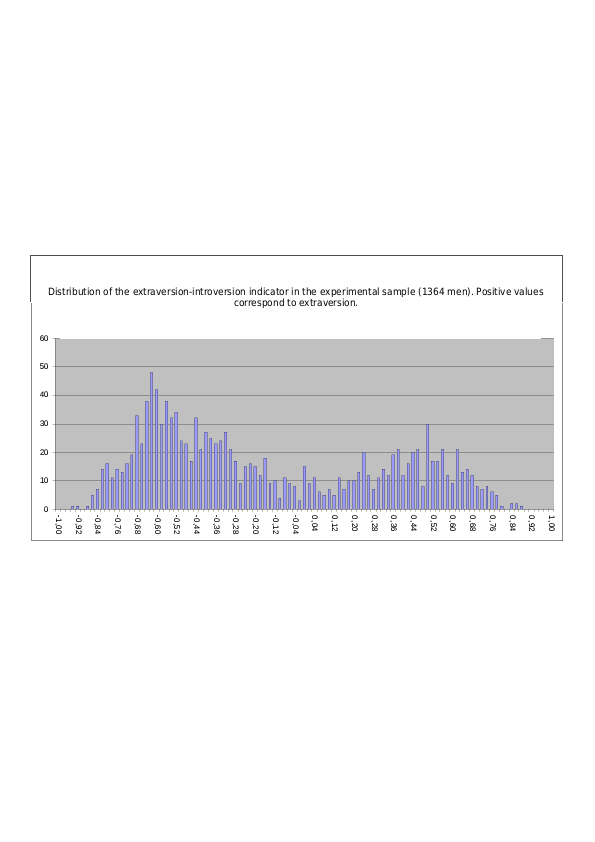
Fig. 14.3.2. Distribution of verticity magnitude. Positive values correspond to extroverts. Female sample (4077 women)
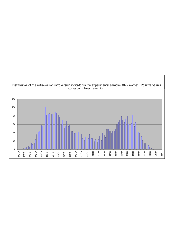
Fig. 14.3.3. Distribution of verticity magnitude. Positive values correspond to extroverts. Mixed sample (1364 men + 4077 women)
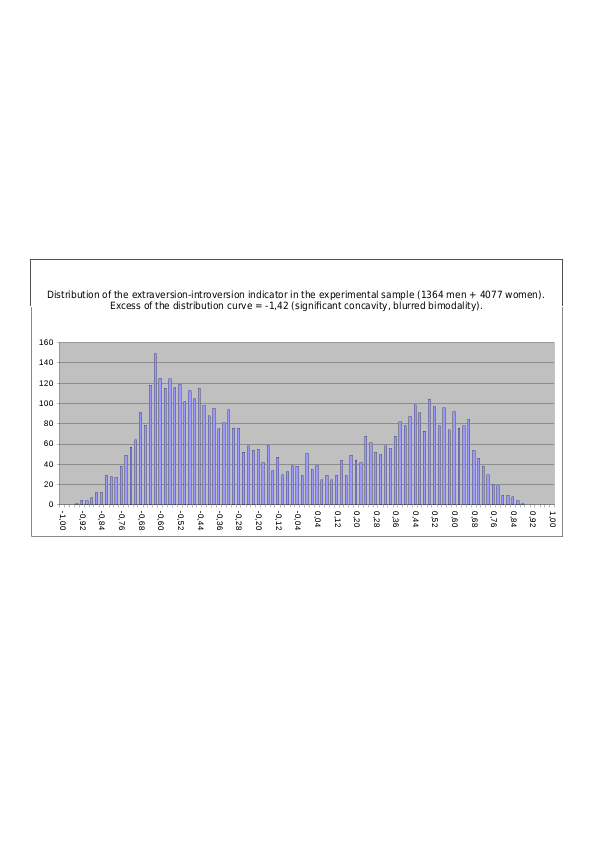
Distribution in the experimental sample of 5441 people of the magnitude of the extraversion-introversion trait calculated from the subjects’ type profiles – when variance-based type commonalities are used in the type profile and normalized by Method No. 2:
Fig. 14.4.1. Distribution of verticity magnitude. Positive values correspond to extroverts. Male sample (1364 men)
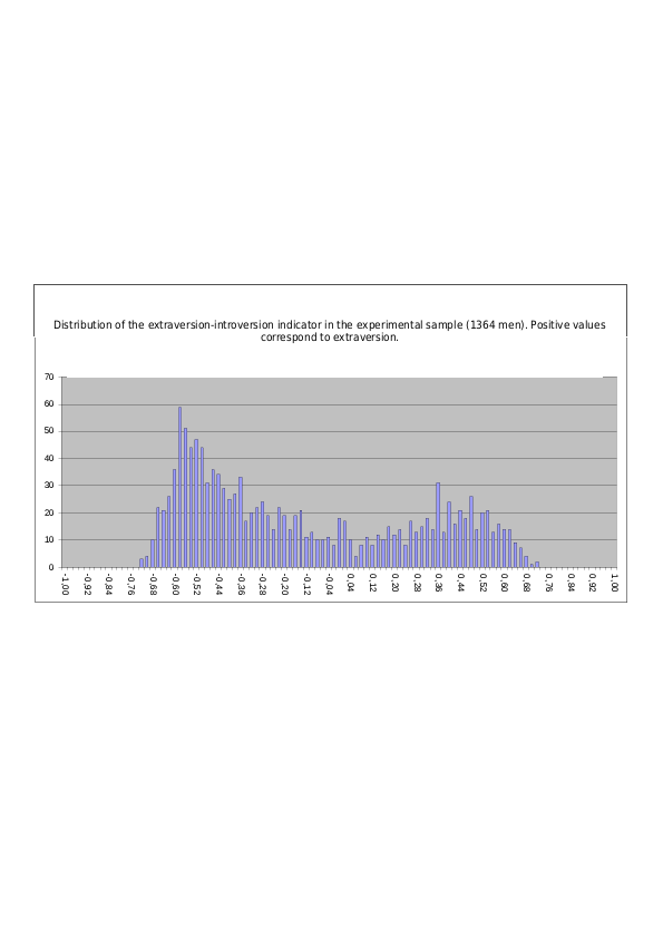
Fig. 14.4.2. Distribution of verticity magnitude. Positive values correspond to extroverts. Female sample (4077 women)
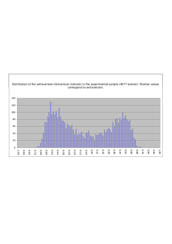
Fig. 14.4.3. Distribution of verticity magnitude. Positive values correspond to extroverts. Mixed sample (1364 men + 4077 women)
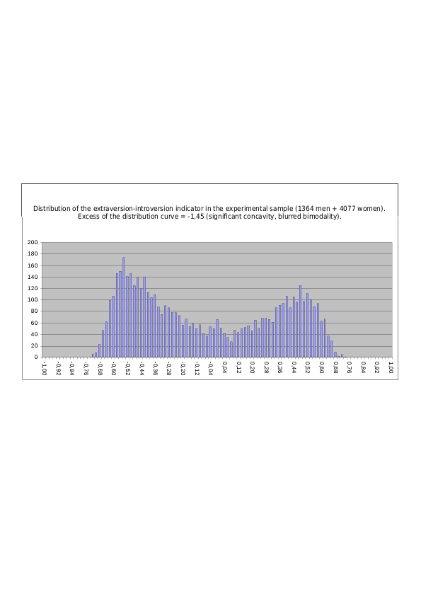
INTUITION-SENSING
Distribution in the experimental sample of 5441 people of the magnitude of the intuition-sensing trait calculated from the subjects’ type profiles – when diagnostic correlations are used in the type profile and normalized by Method No. 1:
Fig. 15.1.1. Distribution of the magnitude of intuition-sensing. Positive values along the X-axis correspond to intuition. Male sample (1364 men)
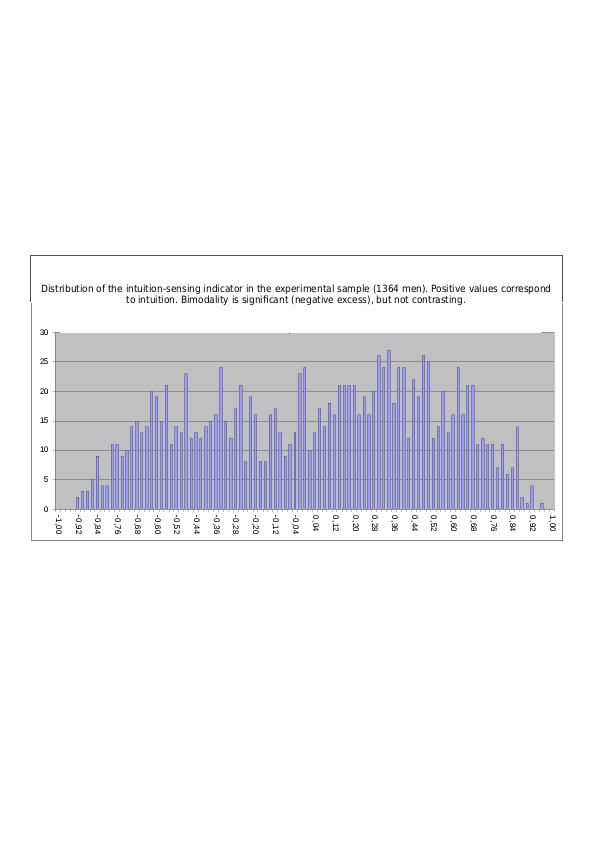
Fig. 15.1.2. Distribution of the magnitude of intuition-sensing. Positive values along the X-axis correspond to intuition. Female sample (4077 women)
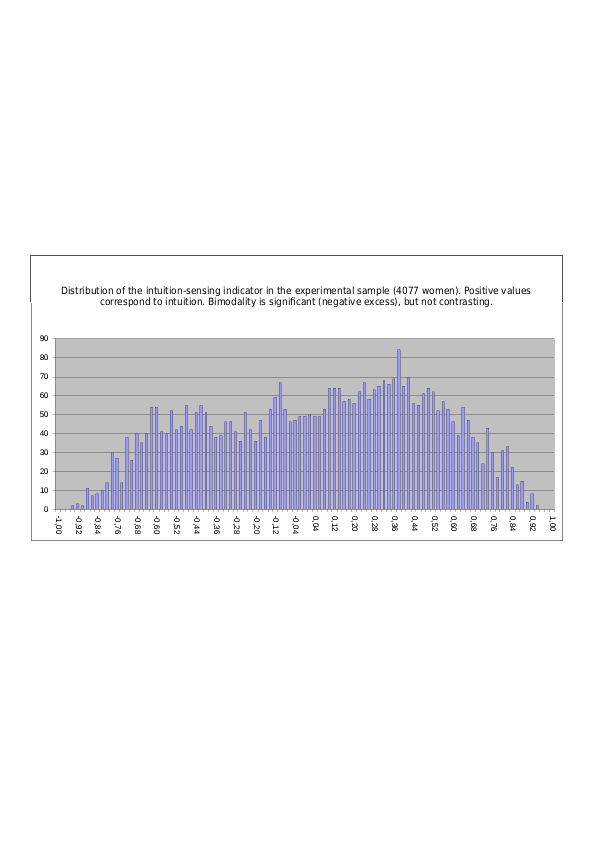
Fig. 15.1.3. Distribution of the magnitude of intuition-sensing. Positive values along the X-axis correspond to intuition. Mixed sample (1364 men + 4077 women)
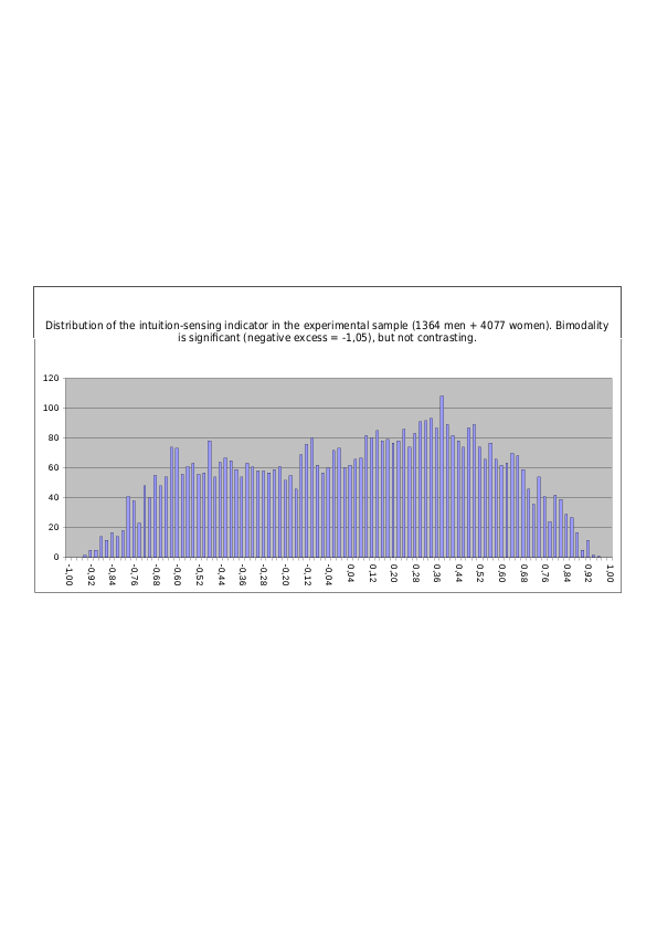
Distribution in the experimental sample of 5441 people of the magnitude of the intuition-sensing trait calculated from the subjects’ type profiles – when diagnostic correlations are used in the type profile and normalized by Method No. 2:
Fig. 15.2.1. Distribution of the magnitude of intuition-sensing. Positive values along the X-axis correspond to intuition. Male sample (1364 men)
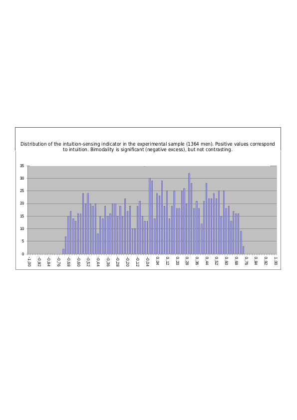
Fig. 15.2.2. Distribution of the magnitude of intuition-sensing. Positive values along the X-axis correspond to intuition. Female sample (4077 women)
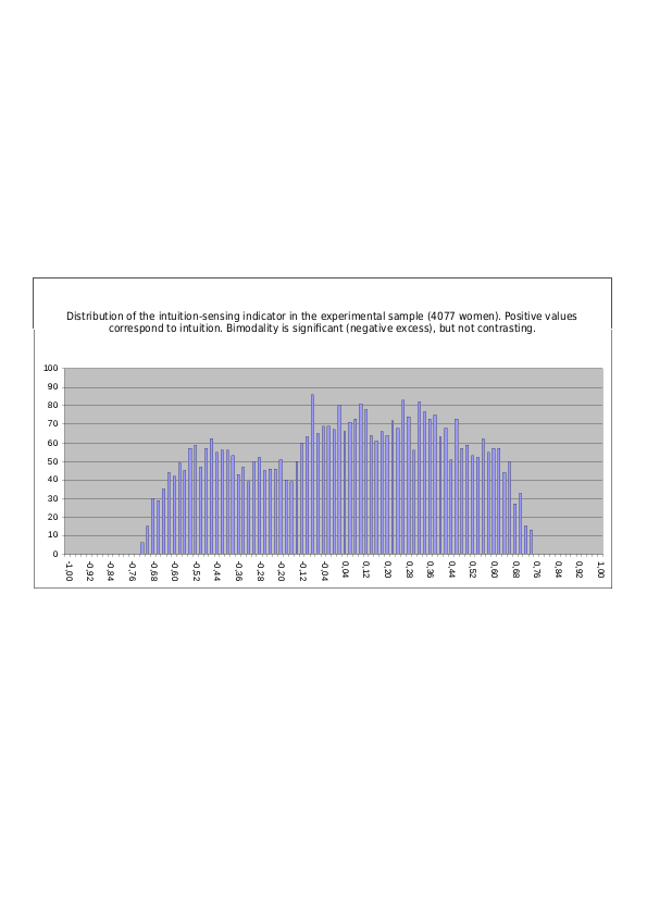
Fig. 15.2.3. Distribution of the magnitude of intuition-sensing. Positive values along the X-axis correspond to intuition. Mixed sample (1364 men + 4077 women)
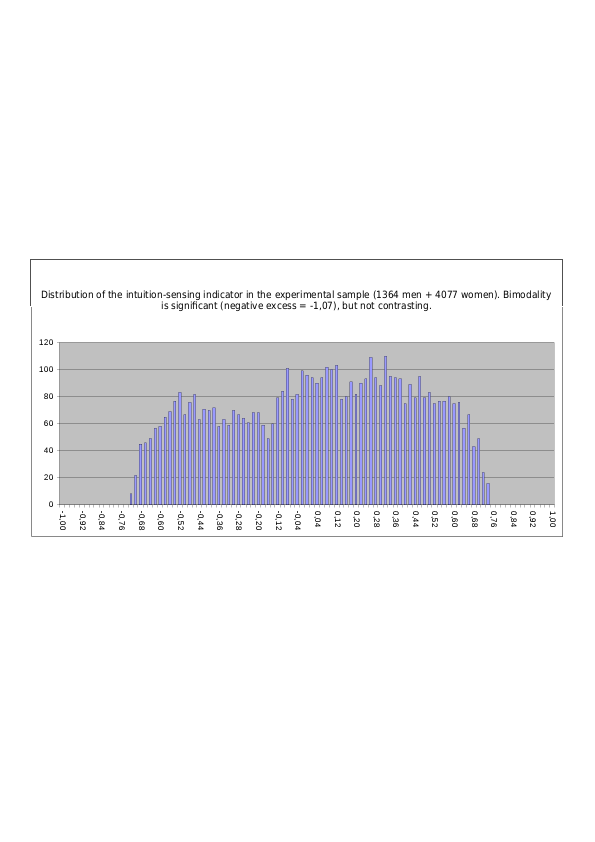
Distribution in the experimental sample of 5441 people of the magnitude of the intuition-sensing trait calculated from the subjects’ type profiles – when variance-based type commonalities are used in the type profile and normalized by Method No. 1:
Fig. 15.3.1. Distribution of the magnitude of intuition-sensing. Positive values along the X-axis correspond to intuition. Male sample (1364 men)
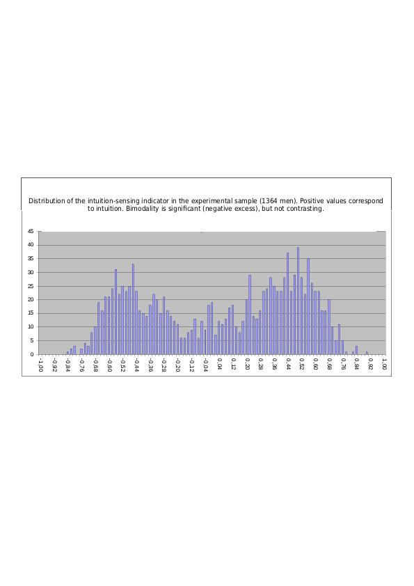
Fig. 15.3.2. Distribution of the magnitude of intuition-sensing. Positive values along the X-axis correspond to intuition. Female sample (4077 women)
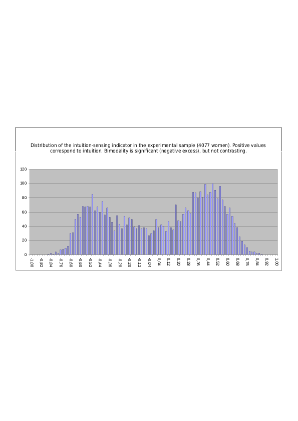
Fig. 15.3.3. Distribution of the magnitude of intuition-sensing. Positive values along the X-axis correspond to intuition. Mixed sample (1364 men + 4077 women)
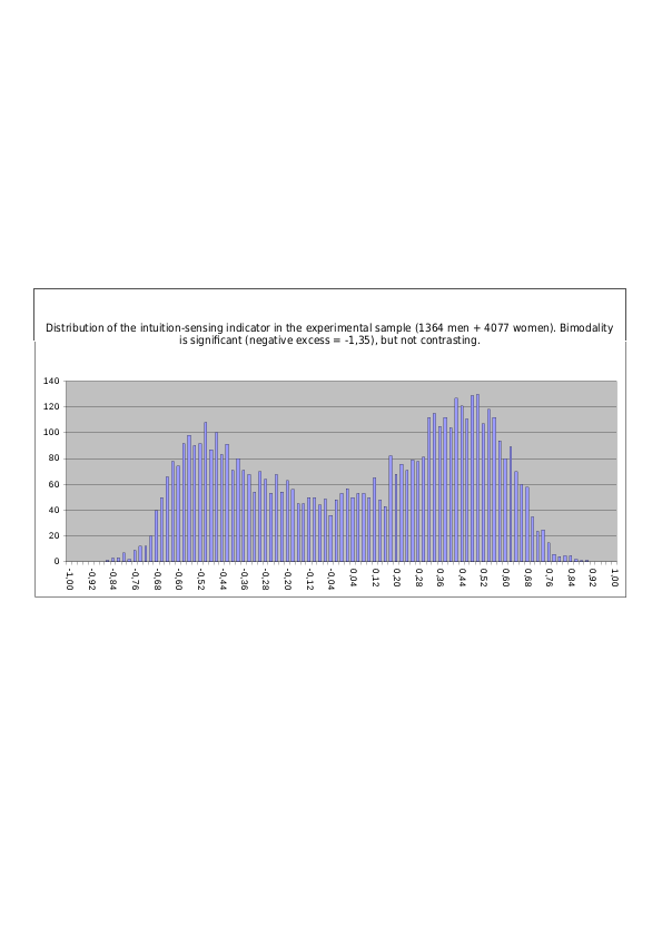
Distribution in the experimental sample of 5441 people of the magnitude of the intuition-sensing trait calculated from the subjects’ type profiles – when variance-based type commonalities are used in the type profile and normalized by Method No. 2:
Fig. 15.4.1. Distribution of the magnitude of intuition-sensing. Positive values along the X-axis correspond to intuition. Male sample (1364 men)
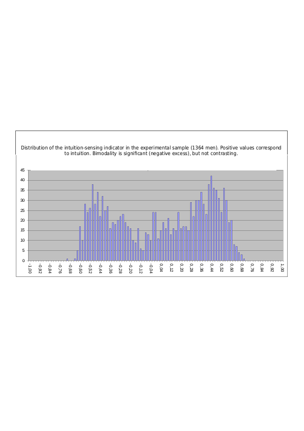
Fig. 15.4.2. Distribution of the magnitude of intuition-sensing. Positive values along the X-axis correspond to intuition. Female sample (4077 women)
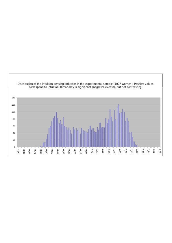
Fig. 15.4.3. Distribution of the magnitude of intuition-sensing. Positive values along the X-axis correspond to intuition. Mixed sample (1364 men + 4077 women)
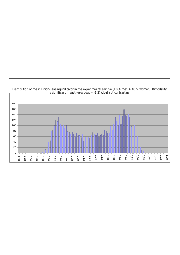
LOGIC-ETHICS
Distribution in the experimental sample of 5441 people of the magnitude of the logic-ethics trait calculated from the subjects’ type profiles – when diagnostic correlations are used in the type profile and normalized by Method No. 1:
Fig. 16.1.1. Distribution of the magnitude of the logic-ethics balance. Positive values along the X-axis correspond to logic. Male sample (1364 men)
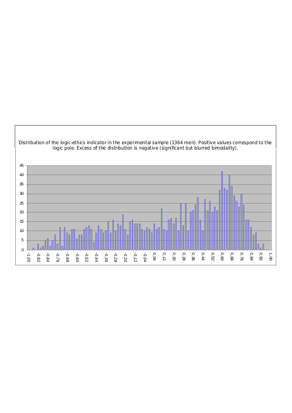
Fig. 16.1.2. Distribution of the magnitude of the logic-ethics balance. Positive values along the X-axis correspond to logic. Female sample (4077 women)
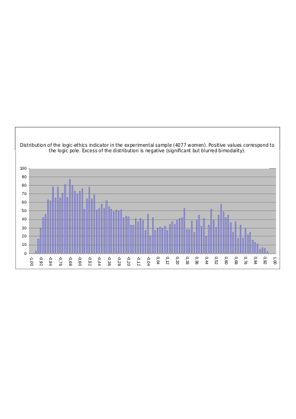
Fig. 16.1.3. Distribution of the magnitude of the logic-ethics balance. Positive values along the X-axis correspond to logic. Mixed sample (1364 men + 4077 women)
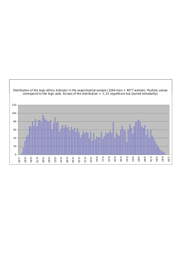
Distribution in the experimental sample of 5441 people of the magnitude of the logic-ethics trait calculated from the subjects’ type profiles – when diagnostic correlations are used in the type profile and normalized by Method No. 2:
Fig. 16.2.1. Distribution of the magnitude of the logic-ethics balance. Positive values along the X-axis correspond to logic. Male sample (1364 men)
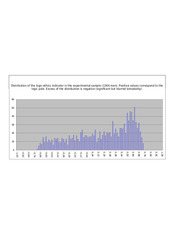
Fig. 16.2.2. Distribution of the magnitude of the logic-ethics balance. Positive values along the X-axis correspond to logic. Female sample (4077 women)
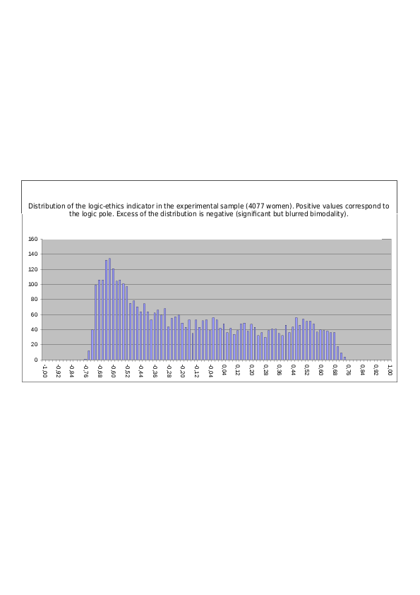
Fig. 16.2.3. Distribution of the magnitude of the logic-ethics balance. Positive values along the X-axis correspond to logic. Mixed sample (1364 men + 4077 women)
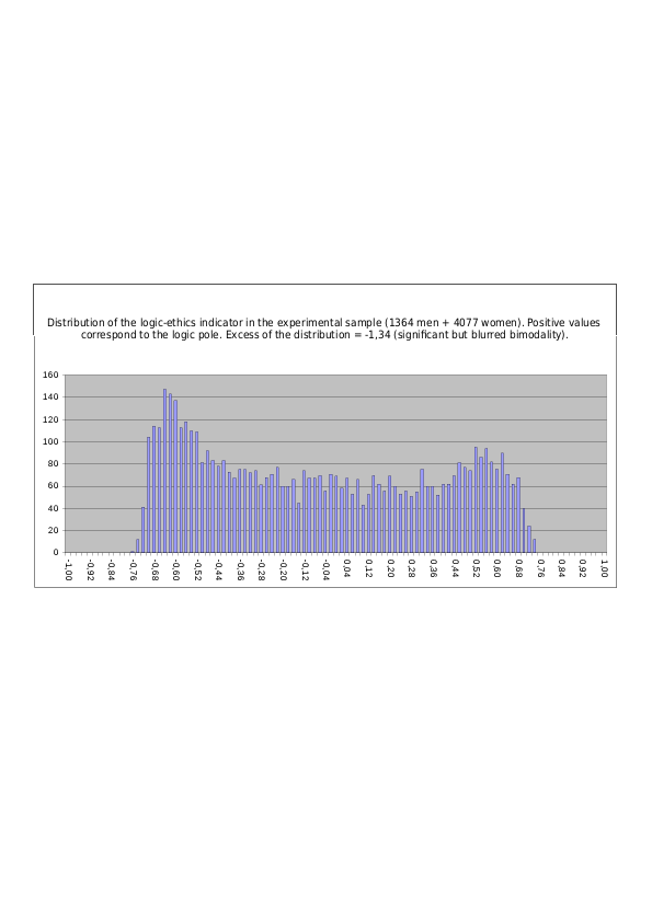
Distribution in the experimental sample of 5441 people of the magnitude of the logic-ethics trait calculated from the subjects’ type profiles – when variance-based type commonalities are used in the type profile and normalized by Method No. 1:
Fig. 16.3..1. Distribution of the magnitude of the logic-ethics balance. Positive values along the X-axis correspond to logic. Male sample (1364 men)
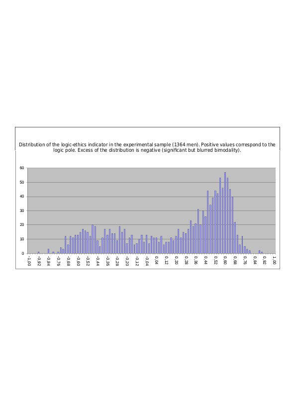
Fig. 16.3.2. Distribution of the magnitude of the logic-ethics balance. Positive values along the X-axis correspond to logic. Female sample (4077 women)
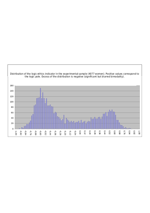
Fig. 16.3.3. Distribution of the magnitude of the logic-ethics balance. Positive values along the X-axis correspond to logic. Mixed sample (1364 men + 4077 women)
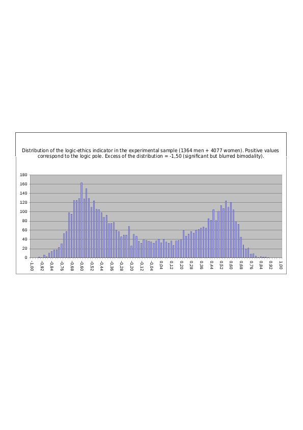
Distribution in the experimental sample of 5441 people of the magnitude of the logic-ethics trait calculated from the subjects’ type profiles – when variance-based type commonalities are used in the type profile and normalized by Method No. 2:
Fig. 16.4.1. Distribution of the magnitude of the logic-ethics balance. Positive values along the X-axis correspond to logic. Male sample (1364 men)
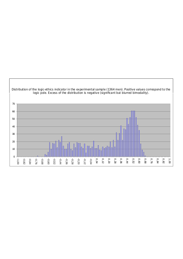
Fig. 16.4.2. Distribution of the magnitude of the logic-ethics balance. Positive values along the X-axis correspond to logic. Female sample (4077 women)
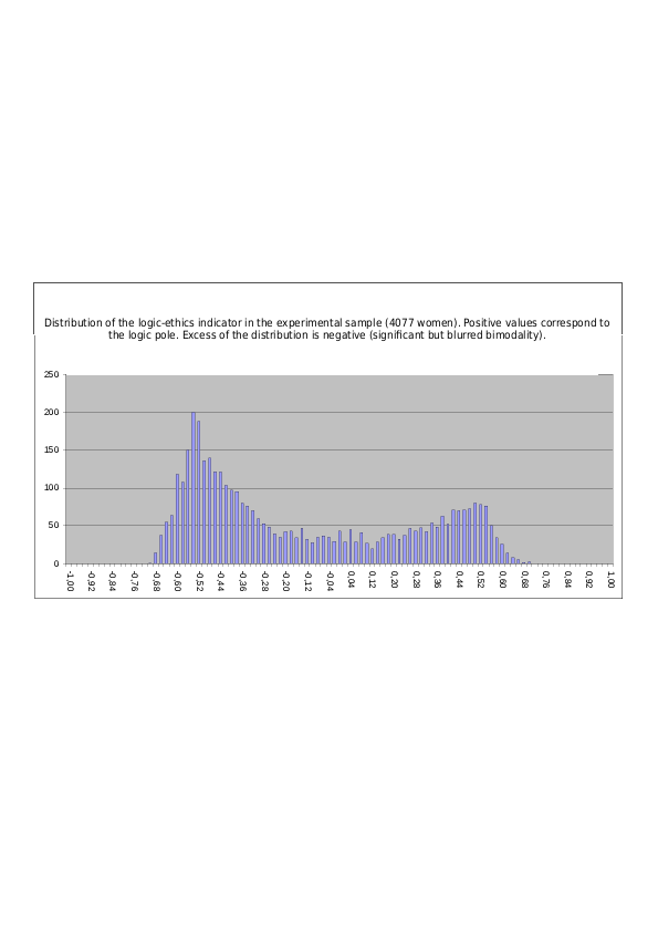
Fig. 16.4.3. Distribution of the magnitude of the logic-ethics balance. Positive values along the X-axis correspond to logic. Mixed sample (1364 men + 4077 women)
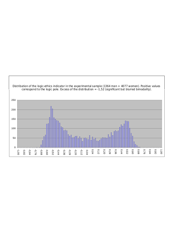
IRRATIONALITY-RATIONALITY
Distribution in the experimental sample of 5441 people of the magnitude of the irrationality-rationality trait calculated from the subjects’ type profiles – when diagnostic correlations are used in the type profile and normalized by Method No. 1:
Fig. 17.1.1. Distribution of the magnitude of the irrationality-rationality balance. Positive values along the X-axis correspond to irrationality. Male sample (1364 men)
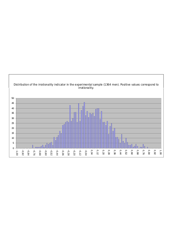
Fig. 17.1.2. Distribution of the magnitude of the irrationality-rationality balance. Positive values along the X-axis correspond to irrationality. Female sample (4077 women)
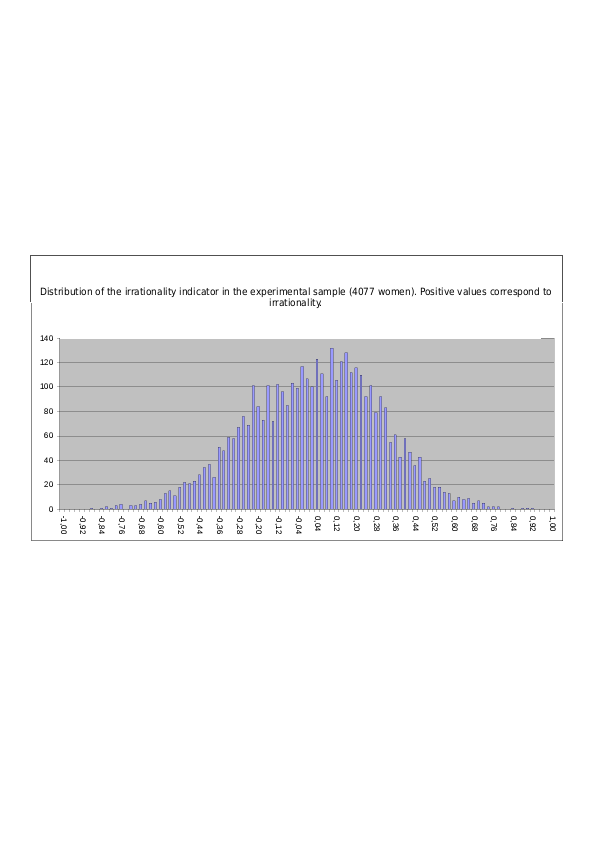
Fig. 17.1.3. Distribution of the magnitude of the irrationality-rationality balance. Positive values along the X-axis correspond to irrationality. Mixed sample (1364 men + 4077 women)
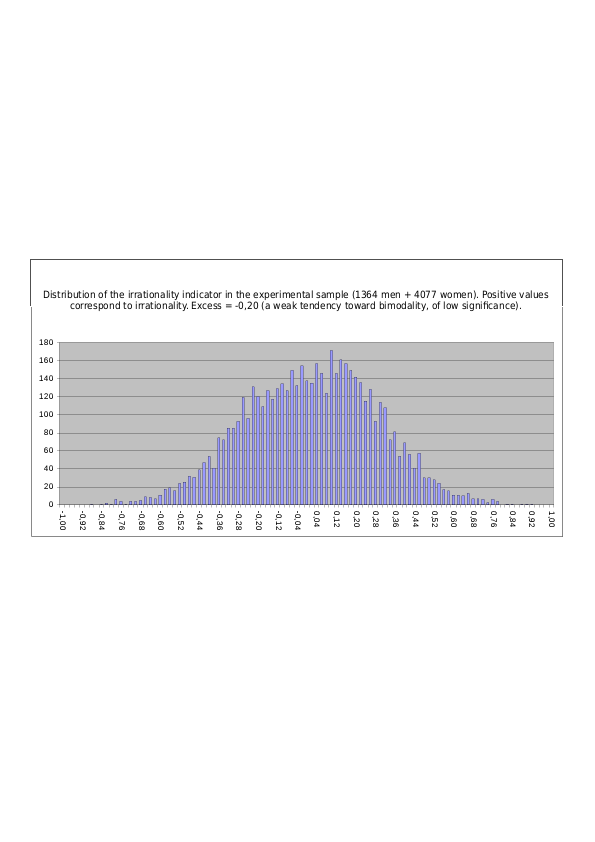
Distribution in the experimental sample of 5441 people of the magnitude of the irrationality-rationality trait calculated from the subjects’ type profiles – when diagnostic correlations are used in the type profile and normalized by Method No. 2:
Fig. 17.2.1. Distribution of the magnitude of the irrationality-rationality balance. Positive values along the X-axis correspond to irrationality. Male sample (1364 men)
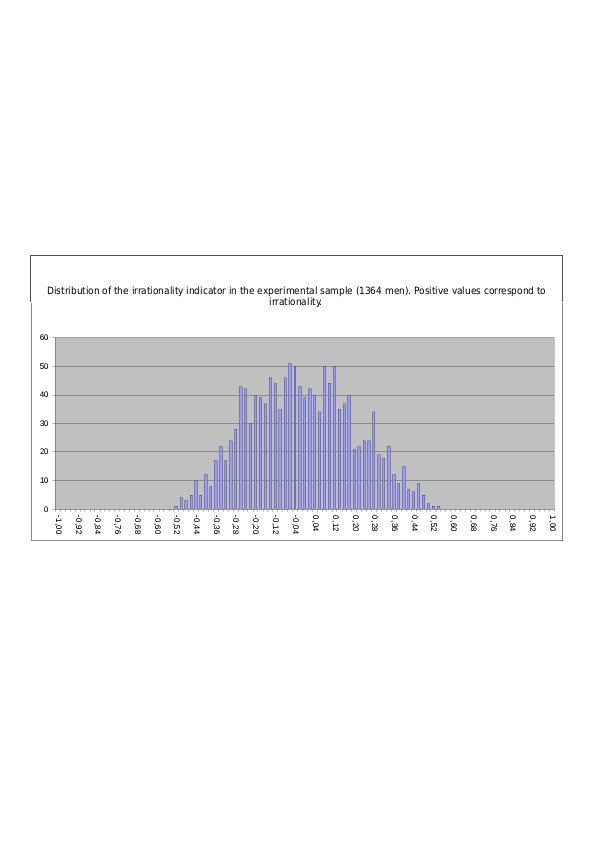
Fig. 17.2.2. Distribution of the magnitude of the irrationality-rationality balance. Positive values along the X-axis correspond to irrationality. Female sample (4077 women)
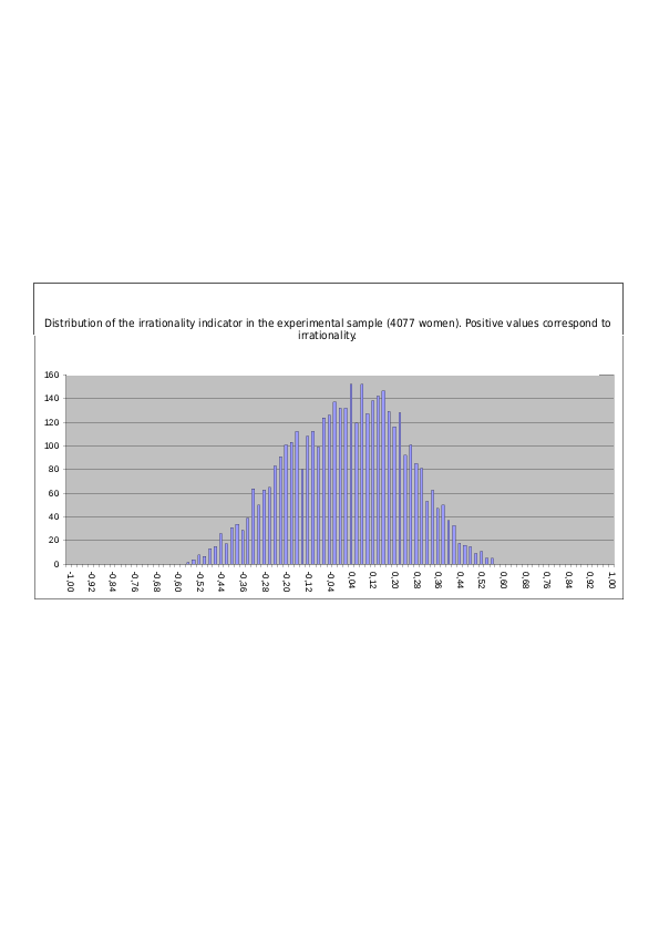
Fig. 17.2.3. Distribution of the magnitude of the irrationality-rationality balance. Positive values along the X-axis correspond to irrationality. Mixed sample (1364 men + 4077 women)
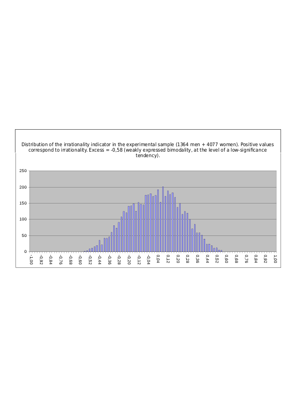
Distribution in the experimental sample of 5441 people of the magnitude of the irrationality-rationality trait calculated from the subjects’ type profiles – when variance-based type commonalities are used in the type profile and normalized by Method No. 1:
Fig. 17.3.1. Distribution of the magnitude of the irrationality-rationality balance. Positive values along the X-axis correspond to irrationality. Male sample (1364 men)
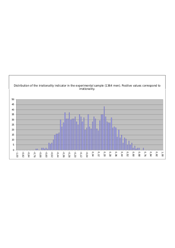
Fig. 17.3.2. Distribution of the magnitude of the irrationality-rationality balance. Positive values along the X-axis correspond to irrationality. Female sample (4077 women)
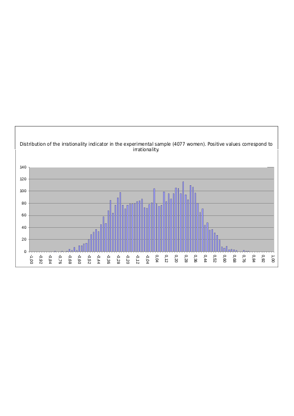
Fig. 17.3.3. Distribution of the magnitude of the irrationality-rationality balance. Positive values along the X-axis correspond to irrationality. Mixed sample (1364 men + 4077 women)
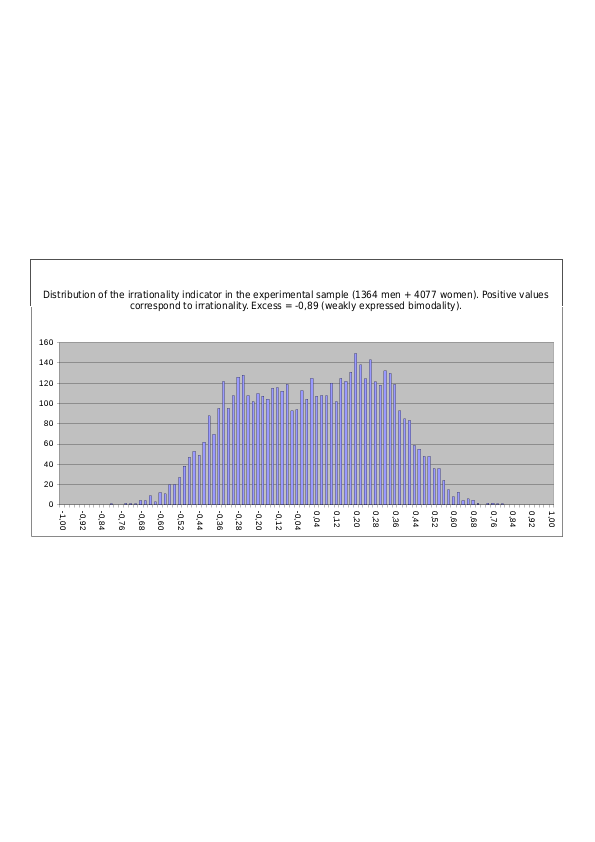
Distribution in the experimental sample of 5441 people of the magnitude of the irrationality-rationality trait calculated from the subjects’ type profiles – when variance-based type commonalities are used in the type profile and normalized by Method No. 2:
Fig. 17.4.1. Distribution of the magnitude of the irrationality-rationality balance. Positive values along the X-axis correspond to irrationality. Male sample (1364 men)
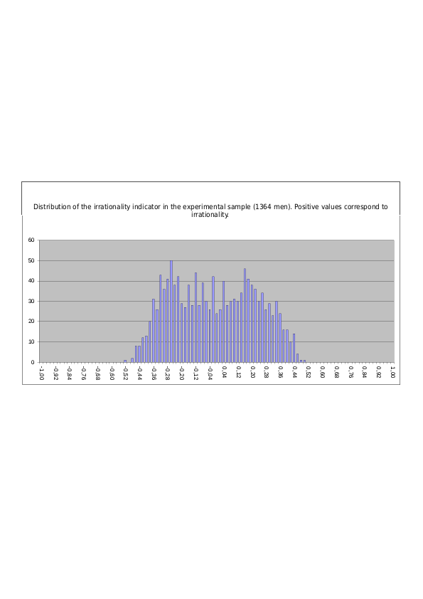
Fig. 17.4.2. Distribution of the magnitude of the irrationality-rationality balance. Positive values along the X-axis correspond to irrationality. Female sample (4077 women)
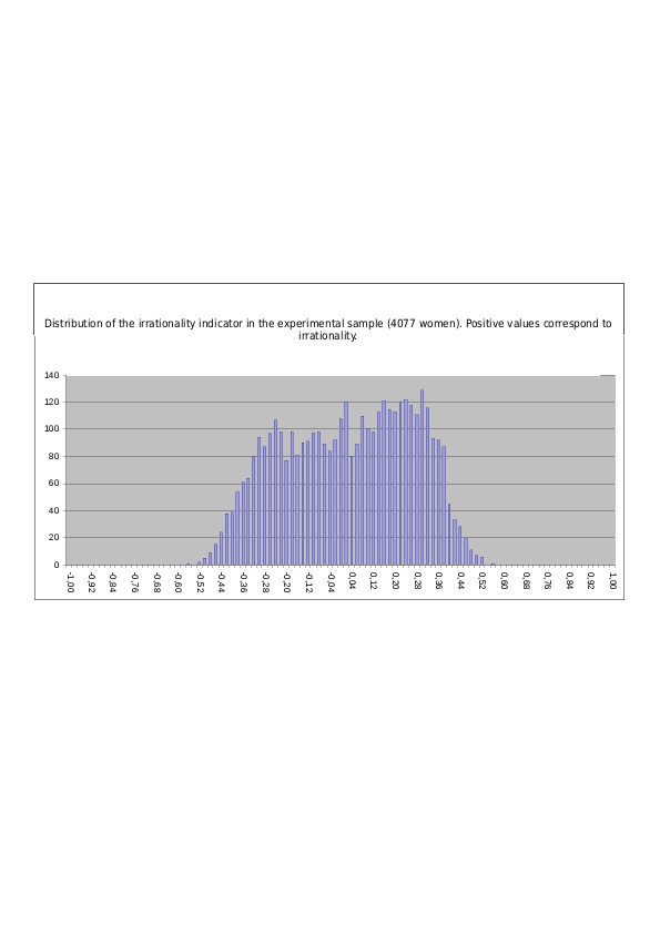
Fig. 17.4.3. Distribution of the magnitude of the irrationality-rationality balance. Positive values along the X-axis correspond to irrationality. Mixed sample (1364 men + 4077 women)
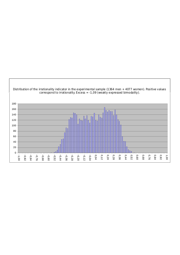
JUDICIOUSNESS-DECISIVENESS
Distribution in the experimental sample of 5441 people of the magnitude of the judiciousness-decisiveness trait calculated from the subjects’ type profiles – when diagnostic correlations are used in the type profile and normalized by Method No. 1:
Fig. 18.1. Distribution of the magnitude of the judiciousness-decisiveness balance. Positive values along the X-axis correspond to judiciousness. Mixed sample (1364 men + 4077 women)
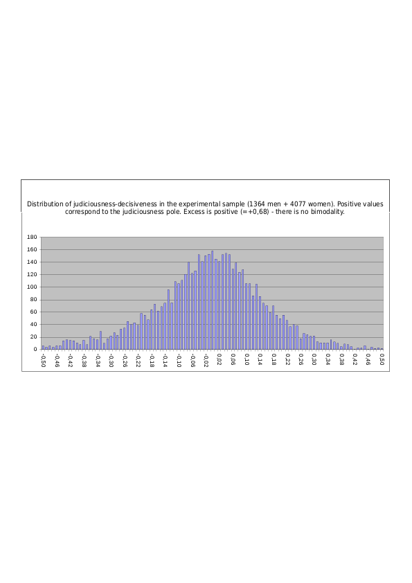
Distribution in the experimental sample of 5441 people of the magnitude of the judiciousness-decisiveness trait calculated from the subjects’ type profiles – when diagnostic correlations are used in the type profile and normalized by Method No. 2:
Fig. 18.2. Distribution of the magnitude of the judiciousness-decisiveness balance. Positive values along the X-axis correspond to judiciousness. Mixed sample (1364 men + 4077 women)
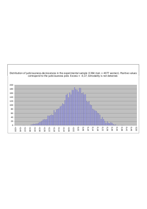
Distribution in the experimental sample of 5441 people of the magnitude of the judiciousness-decisiveness trait calculated from the subjects’ type profiles – when variance-based type commonalities are used in the type profile and normalized by Method No. 1:
Fig. 18.3. Distribution of the magnitude of the judiciousness-decisiveness balance. Positive values along the X-axis correspond to judiciousness. Mixed sample (1364 men + 4077 women)
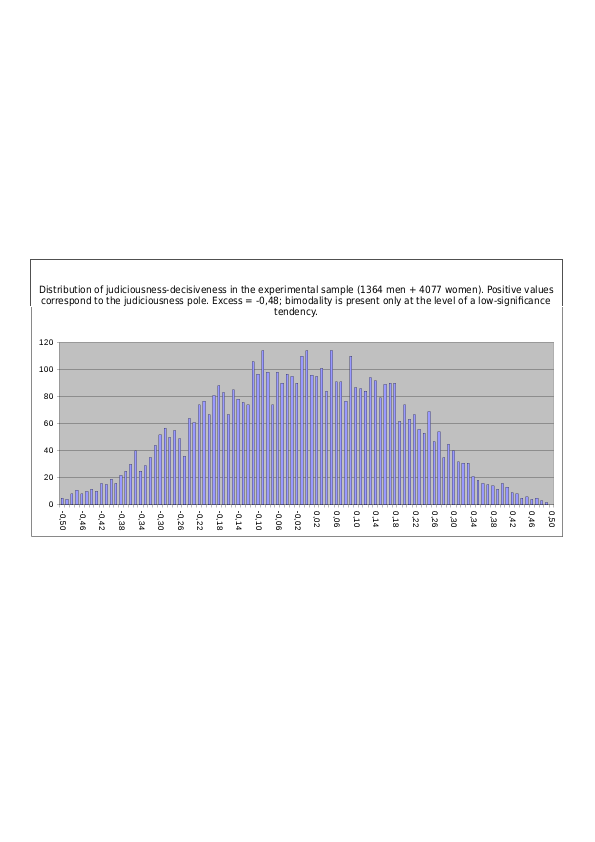
Distribution in the experimental sample of 5441 people of the magnitude of the judiciousness-decisiveness trait calculated from the subjects’ type profiles – when variance-based type commonalities are used in the type profile and normalized by Method No. 2:
Fig. 18.4. Distribution of the magnitude of the judiciousness-decisiveness balance. Positive values along the X-axis correspond to judiciousness. Mixed sample (1364 men + 4077 women)
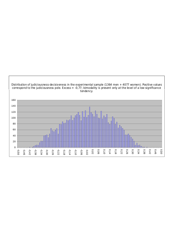
MERRY-SERIOUS
Distribution in the experimental sample of 5441 people of the magnitude of the socionic merry-serious trait calculated from the subjects’ type profiles – when diagnostic correlations are used in the type profile and normalized by Method No. 1:
Fig. 19.1. Distribution of the magnitude of the socionic merry-serious balance. Positive values along the X-axis correspond to the “merry” pole. Mixed sample (1364 men + 4077 women)
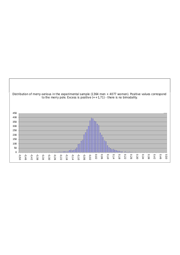
Distribution in the experimental sample of 5441 people of the magnitude of the socionic merry-serious trait calculated from the subjects’ type profiles – when diagnostic correlations are used in the type profile and normalized by Method No. 2:
Fig. 19.2. Distribution of the magnitude of the socionic merry-serious balance. Positive values along the X-axis correspond to the “merry” pole. Mixed sample (1364 men + 4077 women)
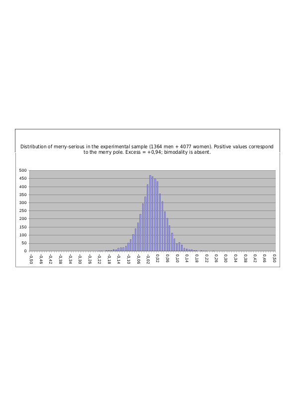
Distribution in the experimental sample of 5441 people of the magnitude of the socionic merry-serious trait calculated from the subjects’ type profiles – when variance-based type commonalities are used in the type profile and normalized by Method No. 1:
Fig. 19.3. Distribution of the magnitude of the socionic merry-serious balance. Positive values along the X-axis correspond to the “merry” pole. Mixed sample (1364 men + 4077 women)
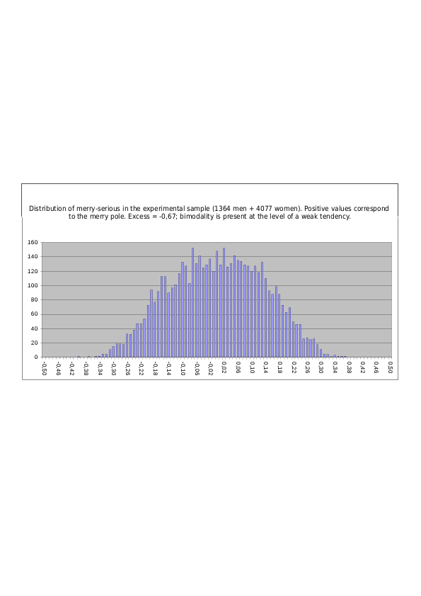
Distribution in the experimental sample of 5441 people of the magnitude of the socionic merry-serious trait calculated from the subjects’ type profiles – when variance-based type commonalities are used in the type profile and normalized by Method No. 2:
Fig. 19.4. Distribution of the magnitude of the socionic merry-serious balance. Positive values along the X-axis correspond to the “merry” pole. Mixed sample (1364 men + 4077 women)
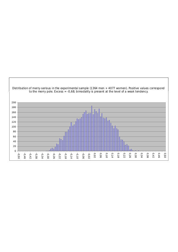
STATIC-DYNAMIC
Distribution in the experimental sample of 5441 people of the magnitude of the socionic static-dynamic trait calculated from the subjects’ type profiles – when diagnostic correlations are used in the type profile and normalized by Method No. 1:
Fig. 20.1. Distribution of the magnitude of the socionic static-dynamic balance. Positive values along the X-axis correspond to the “static” pole. Mixed sample (1364 men + 4077 women)
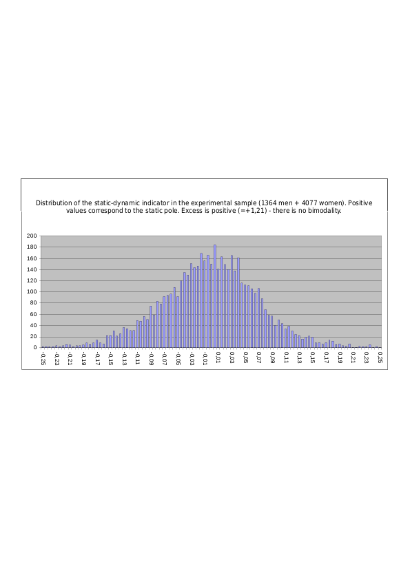
Distribution in the experimental sample of 5441 people of the magnitude of the socionic static-dynamic trait calculated from the subjects’ type profiles – when diagnostic correlations are used in the type profile and normalized by Method No. 2:
Fig. 20.2. Distribution of the magnitude of the socionic static-dynamic balance. Positive values along the X-axis correspond to the “static” pole. Mixed sample (1364 men + 4077 women)
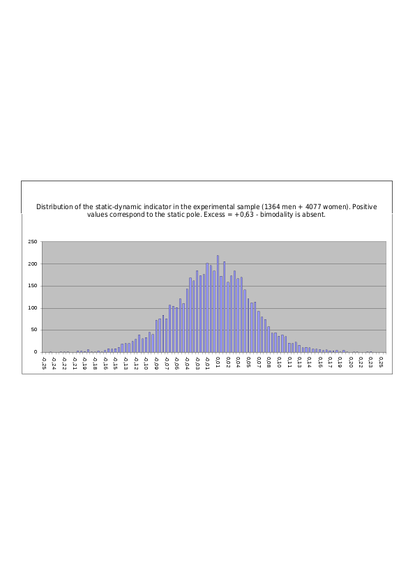
Distribution in the experimental sample of 5441 people of the magnitude of the socionic static-dynamic trait calculated from the subjects’ type profiles – when variance-based type commonalities are used in the type profile and normalized by Method No. 1:
Fig. 20.3. Distribution of the magnitude of the socionic static-dynamic balance. Positive values along the X-axis correspond to the “static” pole. Mixed sample (1364 men + 4077 women)
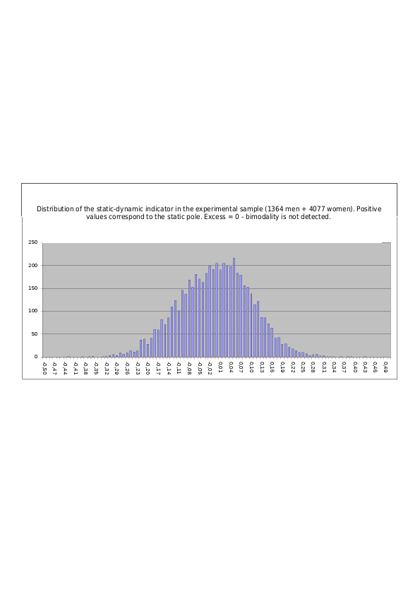
Distribution in the experimental sample of 5441 people of the magnitude of the socionic static-dynamic trait calculated from the subjects’ type profiles – when variance-based type commonalities are used in the type profile and normalized by Method No. 2:
Fig. 20.4. Distribution of the magnitude of the socionic static-dynamic balance. Positive values along the X-axis correspond to the “static” pole. Mixed sample (1364 men + 4077 women)
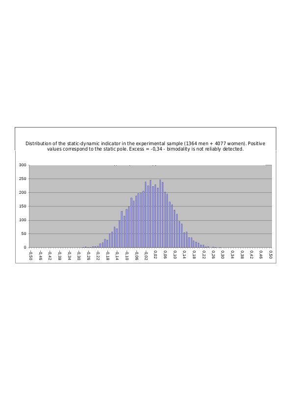
POSITIVISM-NEGATIVISM
Distribution in the experimental sample of 5441 people of the magnitude of the socionic positivism-negativism trait calculated from the subjects’ type profiles – when diagnostic correlations are used in the type profile and normalized by Method No. 1:
Fig. 21.1. Distribution of the magnitude of the socionic positivism-negativism balance. Positive values along the X-axis correspond to the “positivist” pole. Mixed sample (1364 men + 4077 women)
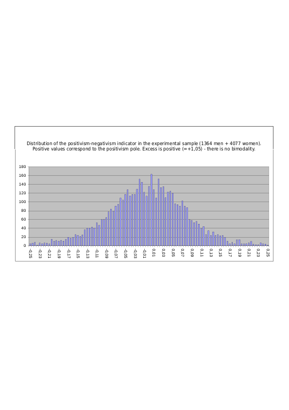
Distribution in the experimental sample of 5441 people of the magnitude of the socionic positivism-negativism trait calculated from the subjects’ type profiles – when diagnostic correlations are used in the type profile and normalized by Method No. 2:
Fig. 21.2. Distribution of the magnitude of the socionic positivism-negativism balance. Positive values along the X-axis correspond to the “positivist” pole. Mixed sample (1364 men + 4077 women)
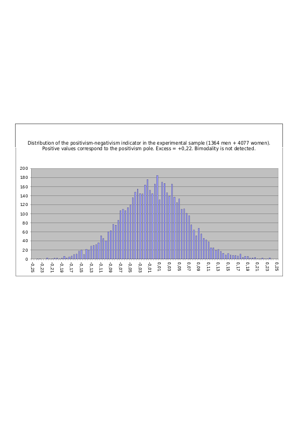
Distribution in the experimental sample of 5441 people of the magnitude of the socionic positivism-negativism trait calculated from the subjects’ type profiles – when variance-based type commonalities are used in the type profile and normalized by Method No. 1:
Fig. 21.3. Distribution of the magnitude of the socionic positivism-negativism balance. Positive values along the X-axis correspond to the “positivist” pole. Mixed sample (1364 men + 4077 women)
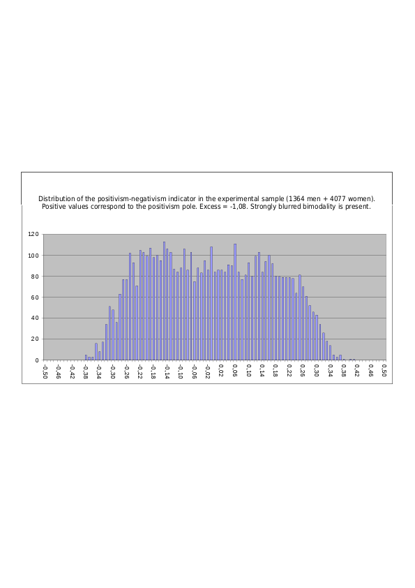
Distribution in the experimental sample of 5441 people of the magnitude of the socionic positivism-negativism trait calculated from the subjects’ type profiles – when variance-based type commonalities are used in the type profile and normalized by Method No. 2:
Fig. 21.4. Distribution of the magnitude of the socionic positivism-negativism balance. Positive values along the X-axis correspond to the “positivist” pole. Mixed sample (1364 men + 4077 women)
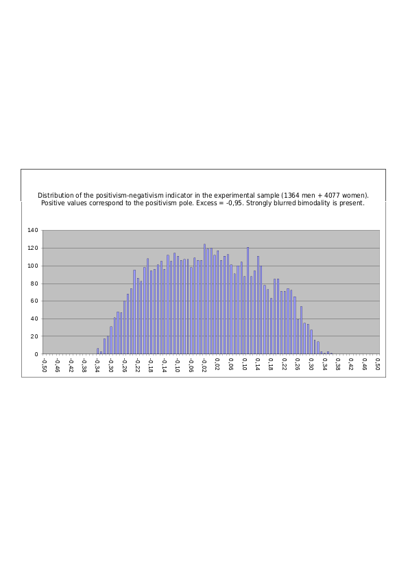
Important Note
After considering the diagrams presented in the part of the article just set out, the behavior of the “positivism-negativism” trait draws particular attention. When this trait is calculated from profiles of diagnostic correlations, its population distribution shows positive excess kurtosis (that is, there is no hint whatsoever of bimodality), yet when calculation shifts to type profiles composed of the squares of correlation coefficients, it suddenly acquires sharply pronounced negative excess kurtosis, almost the same as that of the “strongest” traits – verticity, intuition-sensing, and logic-ethics. What is happening here? Have we discovered some important phenomenon?
Unfortunately, in reality we are dealing with a computational artifact. To understand what happened, examine the first row of Tables 1 and 4, which contains the profile of type loadings for the ILE sociotype (to understand the mechanism of the artifact, the example of this single sociotype is sufficient). The highest loading of ILE is, first, with itself, which is unsurprising – its correlation with itself is equal to the maximum value, one. The next sociotype by contribution to ILE’s loadings is LIE; the correlation of its properties with those of ILE is also very substantial. And there are two more “negative champions” that make the largest negative contributions to the loadings because their properties correlate deeply negatively with the properties of ILE. These are its conflict type ESI and its dual SEI. When we move from Table 1 to Table 4, replacing correlations with squared correlations, all coefficients in each row become even more contrasted. Large coefficients remain large, whereas all the small values close to zero are drawn still closer to zero and almost cease to make any significant contribution to the type profile. Consequently, in Table 4, the properties of the ILE type can, with only a very slight loss of precision, be represented as the sum of the properties of only four types: ILE and LIE taken with a plus sign, and ESI and SEI taken with a minus sign; all the others have almost zero loadings in the profile and remain “outside the boundary.” Now look at Table 6, in which the sociotypes are assigned to the poles of all 15 socionic traits. For which of the 15 traits do ILE and LIE jointly fall on one pole of the trait, while ESI and SEI also jointly fall on the opposite pole? Only four of the 15 traits. These are verticity, intuition-sensing, logic-ethics, and, finally, positivism-negativism. This is why the distributions of these four traits specifically, including positivism-negativism, stretch sharply toward opposite ends of the X-axis when we move from type profiles with diagnostic correlations or numbers proportional to them (Table 1) to profiles with numbers proportional to squared correlations (Table 4). This is why, for these four traits specifically, including positivism-negativism, bipolarity suddenly increases sharply during this transition, as evidenced by the suddenly appearing sharply negative excess kurtosis. The matter can also be viewed from a somewhat different angle: positivism-negativism is equal to the product of verticity, intuition-sensing, and logic-ethics. That is, it is a product of the three strongest socionic traits, moreover traits with negative excess kurtosis. We have encountered a mathematical artifact. No revelation, unfortunately, has occurred.
The example considered with positivism shows that, in terms of the presence or absence of bimodality in the distributions, calculations of traits based not on squared correlations but on the correlations themselves should be more informative – in this case the selectivity of the correlation filters is blurred to a greater degree (almost all psychotypes are taken into account, rather than only two or four), and the probability of artifacts such as the one considered becomes lower. But unfortunately, if we compare the trait-distribution diagrams obtained in this case with those calculated from the squares of the correlation coefficients, we will see that together with the increase in the informativeness of the sought bimodality, the bimodality itself also becomes sharply weaker – traces of it remain, and in attenuated form, only for verticity, intuition-sensing, and logic-ethics.
It appears that, on the basis of the diagrams of trait-magnitude distributions considered in Part 2 of the article just presented, it would be premature to draw a final conclusion about the existence of objective boundaries between sociotypes and between the poles of even the basic socionic traits. On the other hand, nothing at all has yet appeared in the study materials on the basis of which one could conclude that such boundaries are absent and, accordingly, that people are homogeneously distributed in psychological space – if anything, the facts collected tend to indicate the opposite, although far from with perfect incontrovertibility.
Table 6. Sociotypes and poles of socionic traits.
| ILE | LII | SEI | ESE | SLE | LSI | IEI | EIE | SEE | ESI | ILI | LIE | IEE | EII | SLI | LSE | |
|---|---|---|---|---|---|---|---|---|---|---|---|---|---|---|---|---|
| EXTROVERT | 1 | -1 | -1 | 1 | 1 | -1 | -1 | 1 | 1 | -1 | -1 | 1 | 1 | -1 | -1 | 1 |
| INTUITIVE | 1 | 1 | -1 | -1 | -1 | -1 | 1 | 1 | -1 | -1 | 1 | 1 | 1 | 1 | -1 | -1 |
| LOGICAL | 1 | 1 | -1 | -1 | 1 | 1 | -1 | -1 | -1 | -1 | 1 | 1 | -1 | -1 | 1 | 1 |
| IRRATIONAL | 1 | -1 | 1 | -1 | 1 | -1 | 1 | -1 | 1 | -1 | 1 | -1 | 1 | -1 | 1 | -1 |
| JUDICIOUS | 1 | 1 | 1 | 1 | -1 | -1 | -1 | -1 | -1 | -1 | -1 | -1 | 1 | 1 | 1 | 1 |
| CONSTRUCTIVIST | 1 | -1 | -1 | 1 | 1 | -1 | -1 | 1 | -1 | 1 | 1 | -1 | -1 | 1 | 1 | -1 |
| MERRY | 1 | 1 | 1 | 1 | 1 | 1 | 1 | 1 | -1 | -1 | -1 | -1 | -1 | -1 | -1 | -1 |
| TACTICIAN | 1 | -1 | -1 | 1 | -1 | 1 | 1 | -1 | -1 | 1 | 1 | -1 | 1 | -1 | -1 | 1 |
| YIELDING | 1 | -1 | 1 | -1 | 1 | -1 | 1 | -1 | -1 | 1 | -1 | 1 | -1 | 1 | -1 | 1 |
| STATIC | 1 | 1 | -1 | -1 | 1 | 1 | -1 | -1 | 1 | 1 | -1 | -1 | 1 | 1 | -1 | -1 |
| DEMOCRATIC | 1 | 1 | 1 | 1 | -1 | -1 | -1 | -1 | 1 | 1 | 1 | 1 | -1 | -1 | -1 | -1 |
| Questimity | 1 | 1 | -1 | -1 | -1 | -1 | 1 | 1 | 1 | 1 | -1 | -1 | -1 | -1 | 1 | 1 |
| CAREFREE | 1 | -1 | 1 | -1 | -1 | 1 | -1 | 1 | -1 | 1 | -1 | 1 | 1 | -1 | 1 | -1 |
| PROCESS | 1 | -1 | 1 | -1 | -1 | 1 | -1 | 1 | 1 | -1 | 1 | -1 | -1 | 1 | -1 | 1 |
| POSITIVIST | 1 | -1 | -1 | 1 | -1 | 1 | 1 | -1 | 1 | -1 | -1 | 1 | -1 | 1 | 1 | -1 |
Part 3 – Population Distribution of the Magnitude of Socionic Functions Within a TIM
Recall (see work [17]) that the magnitudes of all 8 socionic functions of a subject are calculated as the sum of the products of the coefficients in the row for the corresponding function in Table 7 below by the type loadings in the row of the subject’s type profile. If the type profile is normalized to a unit standard deviation of the type-profile loadings, then, as a result of this multiplication, the functional profile also becomes quasi-normalized, that is, close to a unit standard deviation across the array of values of all 8 functions.
Thus, the results of all subjects in the sample, expressed as normalized type profiles, can be transformed into the functional profiles of those subjects, after which, naturally, diagrams can be constructed for the distribution of function magnitudes in the experimental sample, depending on the names of the functions, their position within the TIM, etc.
Table 7. Coefficients for calculating function magnitudes from a subject’s type profile (a function is calculated as the sum of the products of the elements of the corresponding row of the present table by the row of type-profile loadings). To calculate the values of functions within a particular “standard” TIM, the corresponding row of Table 7 is multiplied (that is, the sum of products is found) by the row from Table 1 or Table 4 corresponding to the required TIM (depending on whether the type profile is used in the metric of diagnostic correlations or in the metric of their squares, that is, the so-called “type commonalities”).
| ILE | LII | SEI | ESE | SLE | LSI | IEI | EIE | SEE | ESI | ILI | LIE | IEE | EII | SLI | LSE | |
|---|---|---|---|---|---|---|---|---|---|---|---|---|---|---|---|---|
| Ni | -0,0625 | -0,0625 | 0,0107 | -0,2393 | -0,0625 | -0,0625 | 0,3643 | 0,1143 | -0,0625 | -0,0625 | 0,3643 | 0,1143 | -0,0625 | -0,0625 | 0,0107 | -0,2393 |
| Ne | 0,3643 | 0,1143 | -0,0625 | -0,0625 | 0,0107 | -0,2393 | -0,0625 | -0,0625 | 0,0107 | -0,2393 | -0,0625 | -0,0625 | 0,3643 | 0,1143 | -0,0625 | -0,0625 |
| Si | -0,0625 | -0,0625 | 0,3643 | 0,1143 | -0,0625 | -0,0625 | 0,0107 | -0,2393 | -0,0625 | -0,0625 | 0,0107 | -0,2393 | -0,0625 | -0,0625 | 0,3643 | 0,1143 |
| Se | 0,0107 | -0,2393 | -0,0625 | -0,0625 | 0,3643 | 0,1143 | -0,0625 | -0,0625 | 0,3643 | 0,1143 | -0,0625 | -0,0625 | 0,0107 | -0,2393 | -0,0625 | -0,0625 |
| Ti | 0,1143 | 0,3643 | -0,0625 | -0,0625 | 0,1143 | 0,3643 | -0,0625 | -0,0625 | -0,2393 | 0,0107 | -0,0625 | -0,0625 | -0,2393 | 0,0107 | -0,0625 | -0,0625 |
| Te | -0,0625 | -0,0625 | -0,2393 | 0,0107 | -0,0625 | -0,0625 | -0,2393 | 0,0107 | -0,0625 | -0,0625 | 0,1143 | 0,3643 | -0,0625 | -0,0625 | 0,1143 | 0,3643 |
| Fi | -0,2393 | 0,0107 | -0,0625 | -0,0625 | -0,2393 | 0,0107 | -0,0625 | -0,0625 | 0,1143 | 0,3643 | -0,0625 | -0,0625 | 0,1143 | 0,3643 | -0,0625 | -0,0625 |
| Fe | -0,0625 | -0,0625 | 0,1143 | 0,3643 | -0,0625 | -0,0625 | 0,1143 | 0,3643 | -0,0625 | -0,0625 | -0,2393 | 0,0107 | -0,0625 | -0,0625 | -0,2393 | 0,0107 |
Diagrams of the distributions of function magnitudes calculated from type profiles composed of diagnostic correlations normalized by Method No. 1 (to a unit standard deviation of the type-profile loadings). Before construction of the diagrams, all functional profiles (individual sets of 8 functions in the subjects’ TIMs) were additionally normalized (by division by the standard deviation of the functional profile), bringing all functional profiles to a unit standard deviation.
Fig. 22.1. Distribution of the magnitude of the program function in the experimental sample (functions calculated from type profiles of diagnostic correlations normalized by Method No. 1) (1364 men + 4077 women)
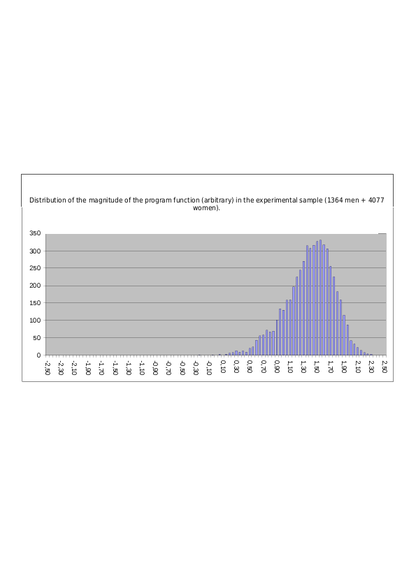
Fig. 22.2. Distribution of the magnitude of the demonstrative function in the experimental sample (functions calculated from type profiles of diagnostic correlations normalized by Method No. 1) (1364 men + 4077 women)
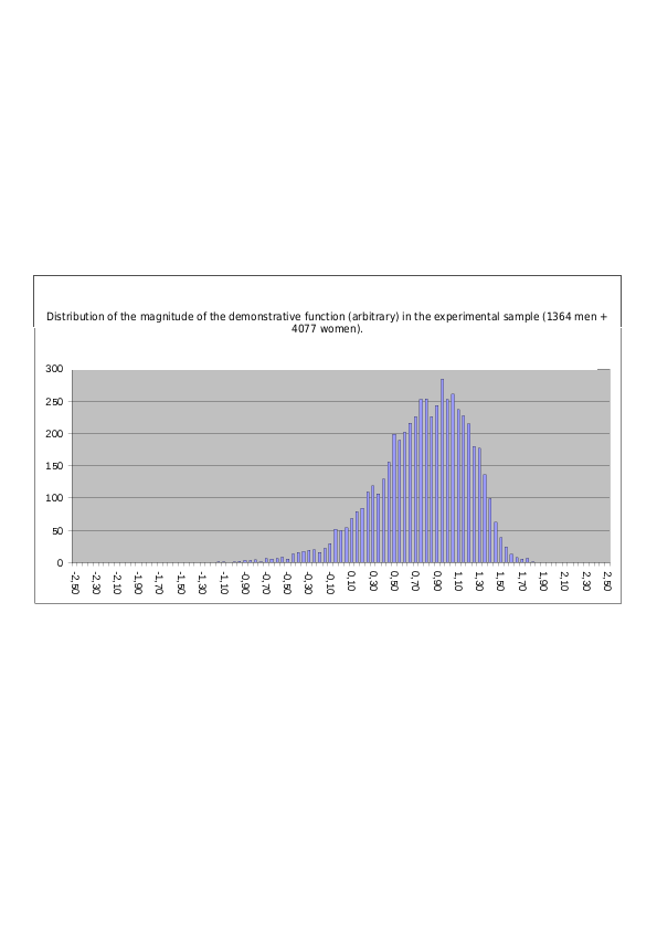
Fig. 22.3. Distribution of the magnitude of the control function in the experimental sample (functions calculated from type profiles of diagnostic correlations normalized by Method No. 1) (1364 men + 4077 women)
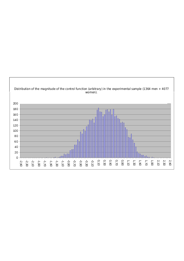
Fig. 22.4. Distribution of the magnitude of the creative function in the experimental sample (functions calculated from type profiles of diagnostic correlations normalized by Method No. 1) (1364 men + 4077 women)
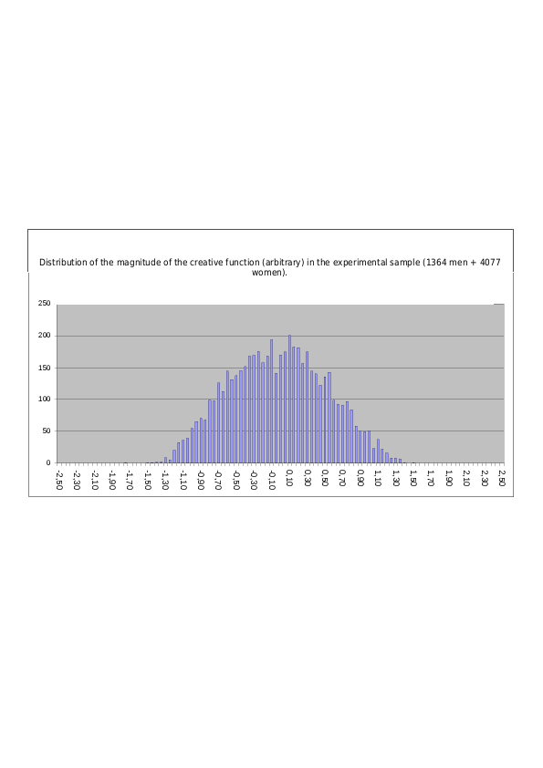
Fig. 22.5. Distribution of the magnitude of the contact function in the experimental sample (functions calculated from type profiles of diagnostic correlations normalized by Method No. 1) (1364 men + 4077 women)
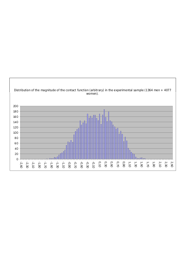
Fig. 22.6. Distribution of the magnitude of the activation function in the experimental sample (functions calculated from type profiles of diagnostic correlations normalized by Method No. 1) (1364 men + 4077 women)
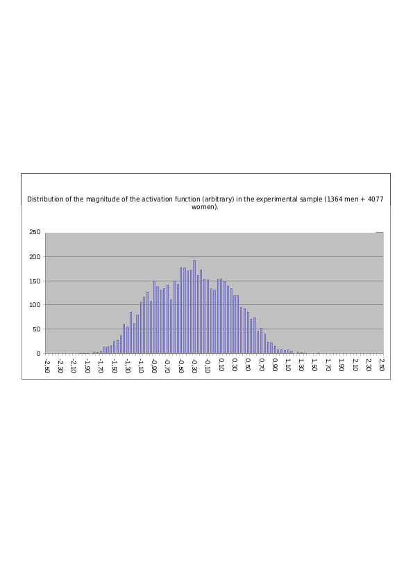
Fig. 22.7. Distribution of the magnitude of the suggestive function in the experimental sample (functions calculated from type profiles of diagnostic correlations normalized by Method No. 1) (1364 men + 4077 women)
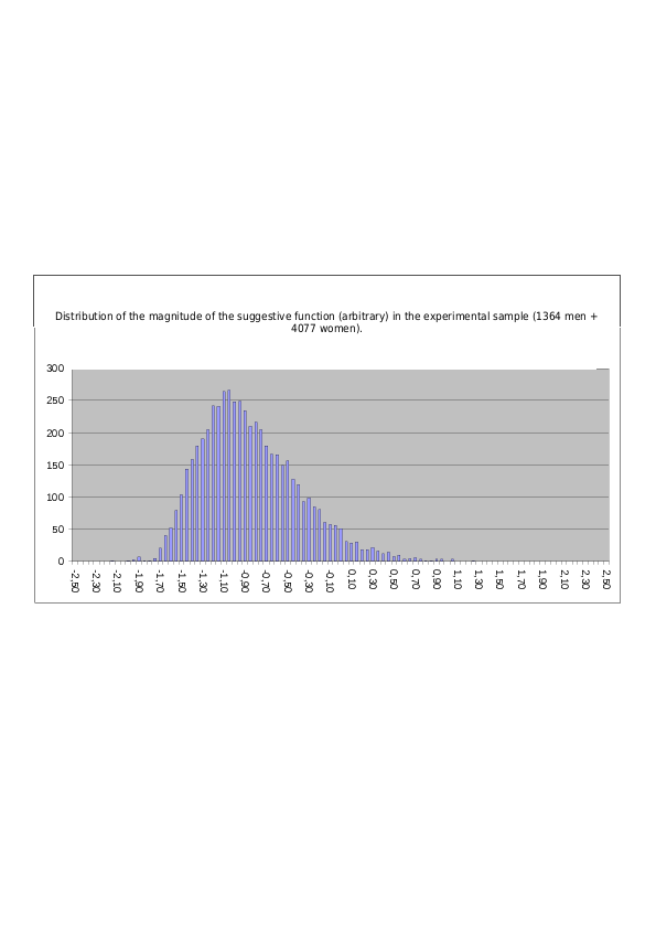
Fig. 22.8. Distribution of the magnitude of the mobilization function in the experimental sample (functions calculated from type profiles of diagnostic correlations normalized by Method No. 1) (1364 men + 4077 women)
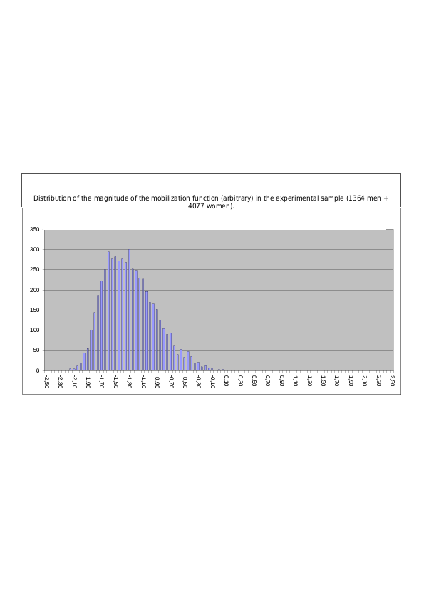
Fig. 23.1. Distribution of function magnitudes (all 8 TIM functions, regardless of their position) in the experimental male sample. Functions calculated from type profiles of diagnostic correlations normalized by Method No. 1 (1364 men)
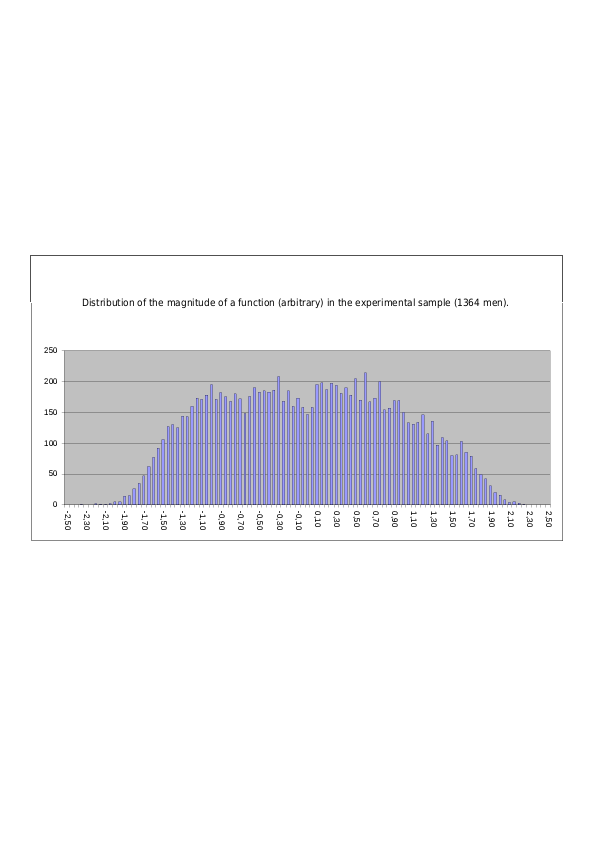
Fig. 23.2. Distribution of function magnitudes (all 8 TIM functions, regardless of their position) in the experimental female sample. Functions calculated from type profiles of diagnostic correlations normalized by Method No. 1 (4077 women)
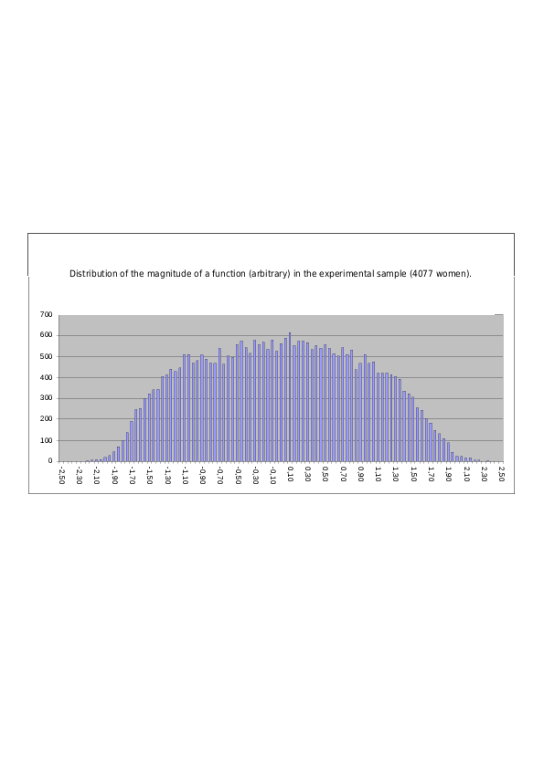
Fig. 23.3. Distribution of function magnitudes (all 8 TIM functions, regardless of their position) in the experimental mixed sample. Functions calculated from type profiles of diagnostic correlations normalized by Method No. 1 (1364 men + 4077 women)
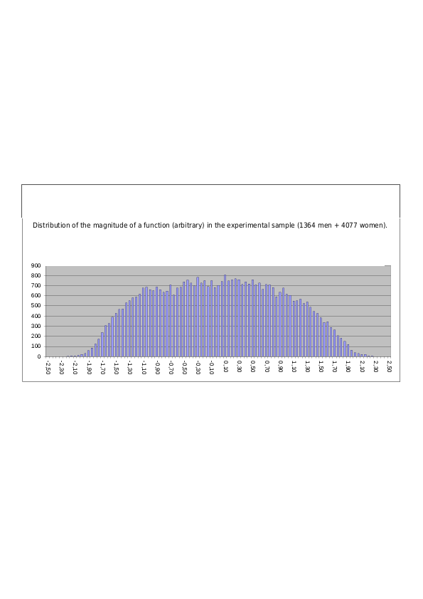
Diagrams of the distributions of function magnitudes calculated from type profiles composed of diagnostic type commonalities (squares of diagnostic correlations with the signs of the correlations), normalized by Method No. 1 (to a unit standard deviation of the type-profile loadings). Before construction of the diagrams, all functional profiles (individual sets of 8 functions in the subjects’ TIMs) were additionally normalized (by division by the standard deviation of the functional profile), bringing all functional profiles to a unit standard deviation.
Fig. 24.1. Distribution of the magnitude of the program function in the experimental sample (functions calculated from type profiles of type commonalities, i.e. squares of diagnostic correlations with signs, normalized by Method No. 1) (1364 men + 4077 women)
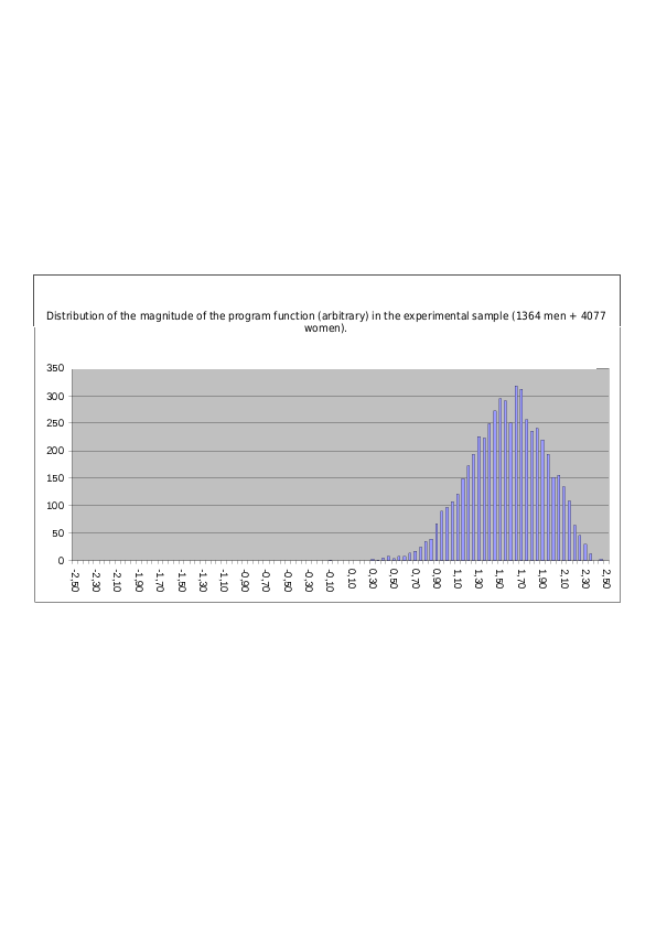
Fig. 24.2. Distribution of the magnitude of the demonstrative function in the experimental sample (functions calculated from type profiles of type commonalities, i.e. squares of diagnostic correlations with signs, normalized by Method No. 1) (1364 men + 4077 women)
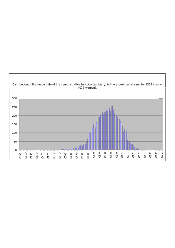
Fig. 24.3. Distribution of the magnitude of the control function in the experimental sample (functions calculated from type profiles of type commonalities, i.e. squares of diagnostic correlations with signs, normalized by Method No. 1) (1364 men + 4077 women)
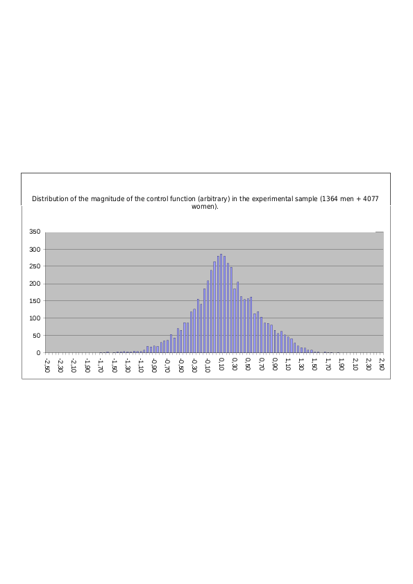
Fig. 24.4. Distribution of the magnitude of the creative function in the experimental sample (functions calculated from type profiles of type commonalities, i.e. squares of diagnostic correlations with signs, normalized by Method No. 1) (1364 men + 4077 women)
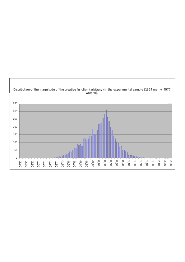
Fig. 24.5. Distribution of the magnitude of the contact function in the experimental sample (functions calculated from type profiles of type commonalities, i.e. squares of diagnostic correlations with signs, normalized by Method No. 1) (1364 men + 4077 women)
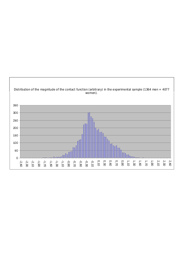
Fig. 24.6. Distribution of the magnitude of the activation function in the experimental sample (functions calculated from type profiles of type commonalities, i.e. squares of diagnostic correlations with signs, normalized by Method No. 1) (1364 men + 4077 women)
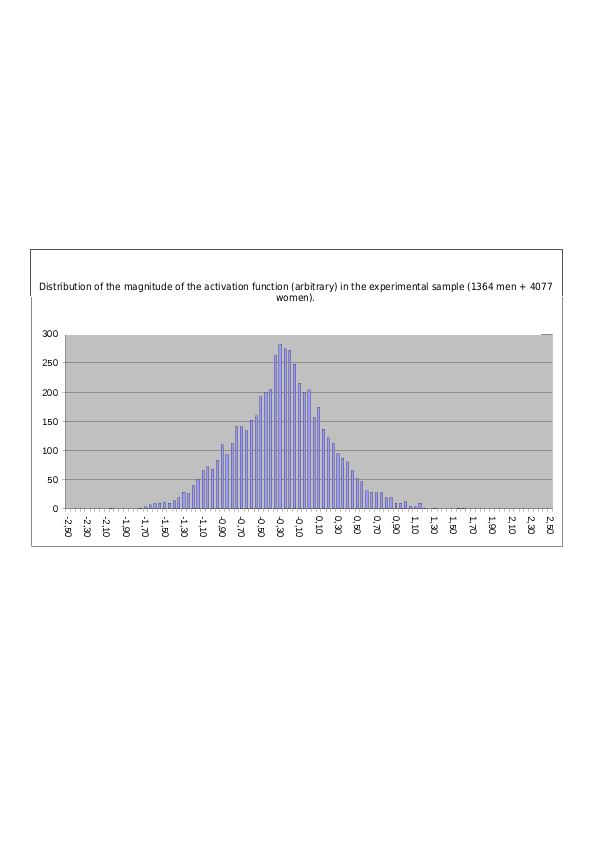
Fig. 24.7. Distribution of the magnitude of the suggestive function in the experimental sample (functions calculated from type profiles of type commonalities, i.e. squares of diagnostic correlations with signs, normalized by Method No. 1) (1364 men + 4077 women)
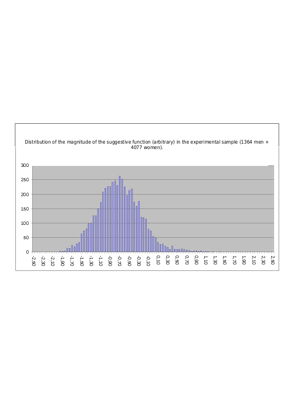
Fig. 24.8. Distribution of the magnitude of the mobilization function in the experimental sample (functions calculated from type profiles of type commonalities, i.e. squares of diagnostic correlations with signs, normalized by Method No. 1) (1364 men + 4077 women)
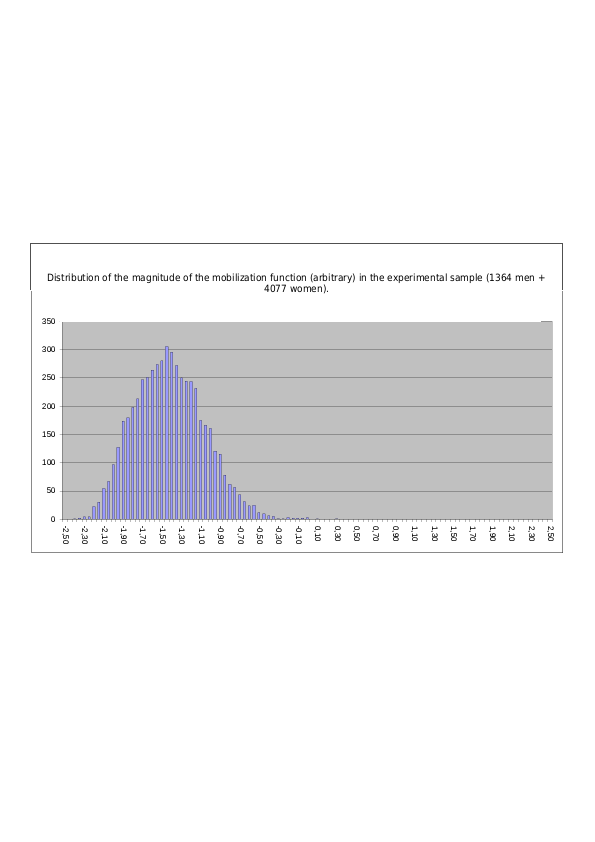
Fig. 25.1. Distribution of function magnitudes (all 8 TIM functions, regardless of their position) in the experimental male sample. Functions calculated from type profiles of type commonalities (squares of diagnostic correlations with signs) normalized by Method No. 1 (1364 men)
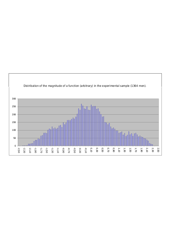
Fig. 25.2. Distribution of function magnitudes (all 8 TIM functions, regardless of their position) in the experimental female sample. Functions calculated from type profiles of type commonalities (squares of diagnostic correlations with signs) normalized by Method No. 1 (4077 women)
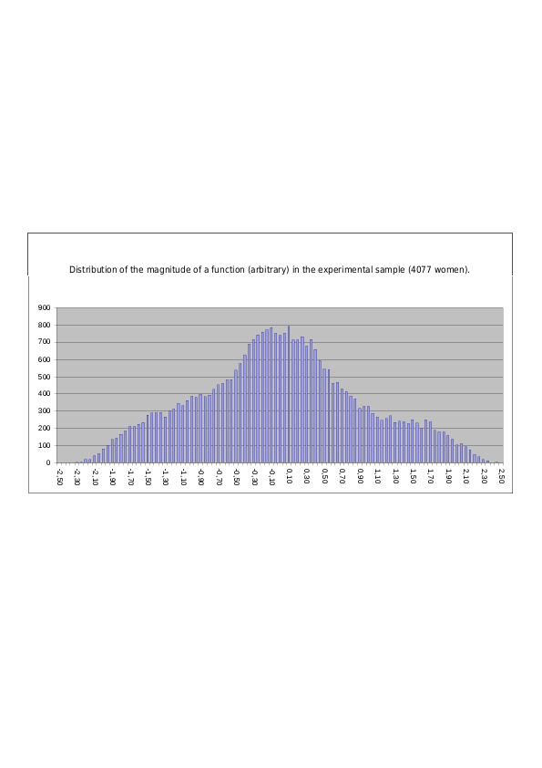
Fig. 25.3. Distribution of function magnitudes (all 8 TIM functions, regardless of their position) in the experimental mixed sample. Functions calculated from type profiles of type commonalities (squares of diagnostic correlations with signs) normalized by Method No. 1 (1364 men + 4077 women)
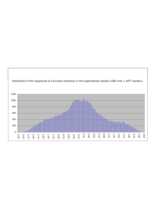
Table 8. Integrated table of characteristics of the population distribution of socionic function magnitudes within a TIM (functions are presented in descending order of their mean magnitudes)
| Accepted numbering of functions in a TIM | Function position | Mean (M+F), functions calculated from type profiles of normalized diagnostic correlations | Median (M+F) | Mode (M+F) | SD (M+F) | SD MEN | SD WOMEN | Mean (M+F), functions calculated from type profiles of normalized variance-based type commonalities (squares of diagnostic correlations with signs) | Median (M+F) | Mode (M+F) | SD (M+F) | SD MEN | SD WOMEN |
|---|---|---|---|---|---|---|---|---|---|---|---|---|---|
| 1 | program function | 1,39 | 1,43 | 1,55 | 0,351 | 0,335 | 0,356 | 1,56 | 1,58 | 1,65 | 0,357 | 0,354 | 0,357 |
| 8 | demonstrative function | 0,77 | 0,82 | 0,95 | 0,428 | 0,428 | 0,429 | 0,58 | 0,61 | 0,75 | 0,442 | 0,440 | 0,443 |
| 7 | control function | 0,31 | 0,33 | 0,10 | 0,562 | 0,555 | 0,564 | 0,17 | 0,14 | 0,10 | 0,475 | 0,461 | 0,480 |
| 2 | creative function | -0,03 | -0,03 | 0,10 | 0,547 | 0,531 | 0,551 | 0,14 | 0,20 | 0,35 | 0,483 | 0,486 | 0,480 |
| 3 | contact function | 0,03 | 0,03 | 0,25 | 0,575 | 0,575 | 0,574 | -0,04 | -0,09 | -0,20 | 0,470 | 0,471 | 0,470 |
| 6 | activation function | -0,33 | -0,33 | -0,30 | 0,577 | 0,571 | 0,579 | -0,28 | -0,27 | -0,30 | 0,476 | 0,472 | 0,478 |
| 5 | suggestive function | -0,85 | -0,92 | -1,05 | 0,459 | 0,451 | 0,461 | -0,71 | -0,73 | -0,70 | 0,451 | 0,450 | 0,451 |
| 4 | mobilization function | -1,29 | -1,33 | -1,30 | 0,377 | 0,358 | 0,383 | -1,42 | -1,44 | -1,45 | 0,361 | 0,357 | 0,362 |
Table 9. Reminder table of the arrangement and names of the positions of socionic functions within a TIM – using the specific TIM ILE as an example
| program | Ne (1) | Ti (2) | creative |
| mobilization | Fi (4) | Se (3) | contact |
| activation | Fe (6) | Si (5) | suggestive |
| control | Ni (7) | Te (8) | demonstrative |
Examination of the diagrams from Fig. 22 through Fig. 25 shows, first, that the “plateau” (a comparatively smoothed flat segment in the shape of the distribution curve) in Fig. 23 is formed by summing the distributions of functions occupying eight different positions (see Figs. 22.1-22.8). The same summation forms the multimodal structure (noticeable “bumpiness”) in the shape of the distribution curve in Fig. 23, especially pronounced for the male sample in Fig. 23.1. The multimodal “bumpiness” in Figs. 23 and 25 is, however, considerably smoothed and blurred, and the reason for this is the very broad distributions of function magnitude in any one of its specific positions. The half-width of the distribution (standard deviation, “SD”) lies in the range from 0,35 for the program function to 0,57 for the contact, activation, and control functions, that is, functions of intermediate magnitude. It must be taken into account, however, that in reality this difference between the half-width of the distribution for functions in their different positions within the TIM is most likely a computational artifact. The reason is that the diagrams were constructed using subjects’ function values in their already normalized functional profiles. In mathematical normalization of profiles (the operation of bringing first the TIM profile and then the functional profile of each individual to a unit standard deviation), the functions deviating most strongly from the mean zero are taken into account with the greatest weight. After normalization, the dispersion of these functions in magnitude is artificially reduced. These are precisely the functions occupying the strongest position (program) and the weakest position (mobilization). For these functions, the dispersion of their magnitudes among subjects is somewhat reduced by normalization in comparison with the real dispersion, whereas for functions differing little from zero it is, conversely, slightly increased. Therefore, it is more correct to speak of a presumed single half-width of the distribution for a function in any of its positions within the TIM, and the correct estimate of this half-width will be the average of the standard deviations calculated for all function positions. As a result, it turns out that the half-width of the distribution (standard deviation) of a socionic function in any one of its specific positions within a TIM is approximately 0,47, and for any specific position of a function within a TIM (program, creative, etc.) this is the true value of population dispersion. Thus, even when a fully definite position of a function within the TIM is fixed (for example, the creative position), variability in the magnitude of the function remains very substantial, such that 34%, or 1/3, of all population cases even remain outside the band of plus or minus 0,47 laid off in both directions from the mean value of the function in the position under consideration. This substantial variability evidently indicates the possibility of very substantial accentuations within the TIM, when for particular individuals the values of the 8 functions within the TIM vary markedly, deviating strongly from the mean population values prescribed to them and fixed for the function positions.
Population distribution of differences between the magnitudes of socionic functions within a TIM in their specified positions. Functions were calculated from type profiles composed of diagnostic correlations normalized by Method No. 1 (to a unit standard deviation of the type-profile loadings). Before construction of the diagrams, all functional profiles (individual sets of 8 functions in the subjects’ TIMs) were additionally normalized (by division by the standard deviation of the functional profile), bringing all functional profiles to a unit standard deviation.
Fig. 26.1. Distribution of differences between the magnitudes of an individual’s program and creative functions in the mixed experimental sample. Functions were calculated on the basis of type profiles of diagnostic correlations; the final functional profiles of eight functions within the TIM were normalized for each subject to a unit standard deviation in the dispersion of the magnitudes of the subject’s eight functions. (1364 men + 4077 women)
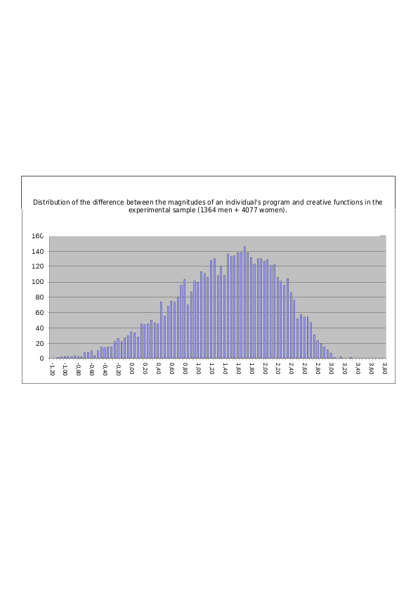
Fig. 26.2. Distribution of differences between the magnitudes of an individual’s program and contact functions in the mixed experimental sample. Functions were calculated on the basis of type profiles of diagnostic correlations; the final functional profiles of eight functions within the TIM were normalized for each subject to a unit standard deviation in the dispersion of the magnitudes of the subject’s eight functions. (1364 men + 4077 women)
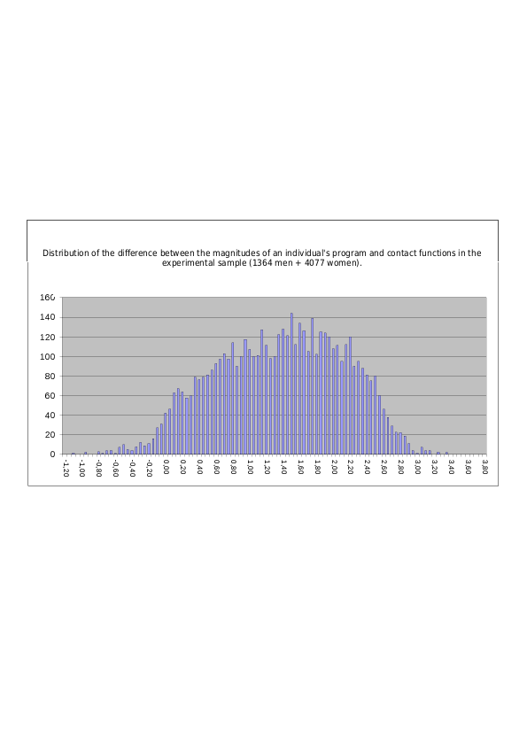
Fig. 26.3. Distribution of differences between the magnitudes of an individual’s creative and contact functions in the mixed experimental sample. Functions were calculated on the basis of type profiles of diagnostic correlations; the final functional profiles of eight functions within the TIM were normalized for each subject to a unit standard deviation in the dispersion of the magnitudes of the subject’s eight functions. (1364 men + 4077 women)
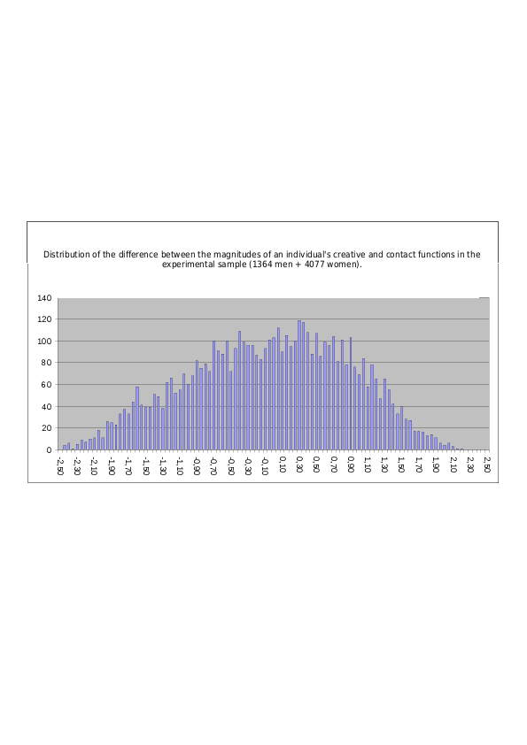
Fig. 26.4. Distribution of differences between the magnitudes of an individual’s creative and mobilization functions in the mixed experimental sample. Functions were calculated on the basis of type profiles of diagnostic correlations; the final functional profiles of eight functions within the TIM were normalized for each subject to a unit standard deviation in the dispersion of the magnitudes of the subject’s eight functions. (1364 men + 4077 women)
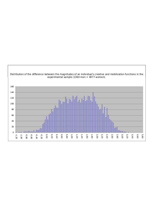
Fig. 26.5. Distribution of differences between the magnitudes of an individual’s contact and mobilization functions in the mixed experimental sample. Functions were calculated on the basis of type profiles of diagnostic correlations; the final functional profiles of eight functions within the TIM were normalized for each subject to a unit standard deviation in the dispersion of the magnitudes of the subject’s eight functions. (1364 men + 4077 women)
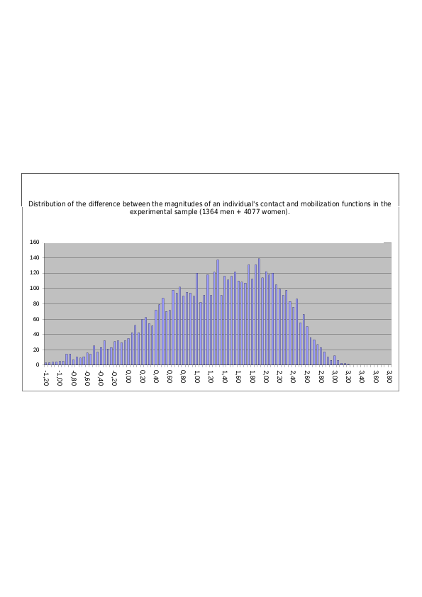
Fig. 26.6. Distribution of differences between the magnitudes of an individual’s program and mobilization functions in the mixed experimental sample. Functions were calculated on the basis of type profiles of diagnostic correlations; the final functional profiles of eight functions within the TIM were normalized for each subject to a unit standard deviation in the dispersion of the magnitudes of the subject’s eight functions. (1364 men + 4077 women)
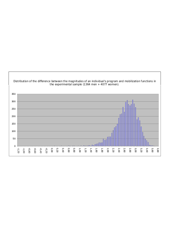
Fig. 26.7. Distribution of differences between the magnitudes of an individual’s program and demonstrative functions in the mixed experimental sample. Functions were calculated on the basis of type profiles of diagnostic correlations; the final functional profiles of eight functions within the TIM were normalized for each subject to a unit standard deviation in the dispersion of the magnitudes of the subject’s eight functions. (1364 men + 4077 women)
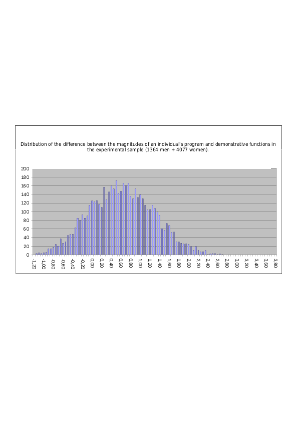
Fig. 26.8. Distribution of differences between the magnitudes of an individual’s demonstrative and control functions in the mixed experimental sample. Functions were calculated on the basis of type profiles of diagnostic correlations; the final functional profiles of eight functions within the TIM were normalized for each subject to a unit standard deviation in the dispersion of the magnitudes of the subject’s eight functions. (1364 men + 4077 women)
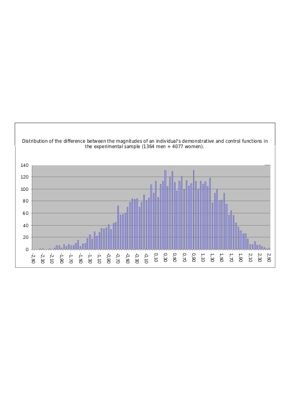
Averaged over the eight function differences presented above, the half-width of the distribution of the difference (the standard deviation of the population distribution of the difference between two functions) is 0,745. Obviously, this is a substantial value, indicating very great freedom in the formation of accentuations within a psychotype. Recall also that the half-width of the distribution of the magnitude of each function separately is, on average, 0,47.
Conclusions
Possible type accentuations have a finite fixed “radius” in the metric of normalized diagnostic correlations (see the half-width of the population distribution of the difference between normalized diagnostic correlations, columns 3 and 4 in Table 3). Thus, the possible effective radius of accentuation is constant and does not depend on the type toward which the accentuation occurs (quasi-identical type, kindred type, conflict type, etc.). If the distance between types (columns 1 and 2 in Table 3) exceeds this fixed radius by more than threefold, the boundary zone between the types becomes empty, practically free of people. If, however, the distance between types in the metric of diagnostic correlations is less than three times the radius of possible type accentuation, then the boundary between the types is not empty; people are found whose accentuations place them even directly on this boundary. Their number is greater, the smaller the ratio of the distance between types to the constant radius of accentuation.
The 16 socionic types in the metric of diagnostic correlations are separated from one another by natural boundaries. Although at a small distance between types accentuations may “creep” even directly onto this boundary, the boundary between the types does not thereby lose its objective character, because the density on it of people who, owing to their accentuations, fall into this boundary zone is nevertheless minimal; it is several times lower than the density of people filling the “core” of a type.
The boundary between quasi-identical types is the most “blurred,” owing to their proximity to one another in the metric of diagnostic correlations. The boundary between conflict types is the most clearly expressed, and even has a broad “forbidden band,” owing to their considerable distance from one another in the metric of diagnostic correlations.
Nevertheless, on the basis of the results of the present study, the separate existence of the 16 socionic types cannot be regarded as fully confirmed. It is confirmed only in the metric of diagnostic correlations, but from a mathematical point of view these correlations themselves are broadband filters locally tuned to particular regions of psychological space; the transmission of these filters, and the magnitude of the observed correlation, decline fairly rapidly with distance from the tuning point. It therefore cannot be completely excluded that the resulting “objective” boundaries between types are merely an artifact of the mathematical calculation method.
For final conclusions regarding the separateness or non-separateness of socionic types, calculations must be performed in the metric of continuous diagnostic scales rather than correlation coefficients. What is a continuous diagnostic scale and how can it be used, for example, to study the transition between LII and ILI? For LII, the questionnaire items to which this type specifically gives the highest responses are selected. The same is done for ILI. Positive responses to each type’s own set of exclusive items are summed with the necessary weighting coefficients, which in turn depend on the degree of exclusivity of these items for the type. These are continuous diagnostic scales, created separately for each of the 16 types. The types themselves, including LII and ILI, are, however, diagnosed in subjects by the usual most accurate method, using the diagnostic-correlation procedure. The sums of responses on the scales are normalized to a unit standard deviation, each on an array of responses from representatives of its “own” type only. The corresponding sums are then calculated for all subjects in the sample. After this, in the array of LII subjects one can compare the results of the continuous diagnostic scales measuring the expression of LII and ILI properties; the same can be done for the array of ILI subjects; and then, from the distribution of the magnitude of the difference between the results of the two diagnostic scales, the boundary zone between these two psychotypes specifically, LII and ILI, can be analyzed in the combined array of representatives of these two psychotypes. The advantage of this approach is that continuous diagnostic scales, unlike correlation coefficients, are not locally tuned to a particular zone of psychological space and, moreover, have a linear mathematical nature.
The results obtained in Part 3 of the present article indicate the possibility of very substantial variation of socionic functions within a TIM in their magnitude relative to one another, which confirms the presence in the population of substantial socionic accentuations corresponding to the strengthening or weakening of certain functions within the TIM. On the other hand, the distribution of the magnitudes of all functions within the TIM has, in the population, a texture close to a jagged multimodal one, that is, population variation of function magnitudes around their position-dependent mean values is nevertheless limited.
In the metric of diagnostic correlations, weakly expressed bimodality is found only for the poles of the socionic traits extroverts-introverts, intuitives-sensors, and logicals-ethicals; for the other traits, bimodality was not found even in the metric of diagnostic correlations. For final conclusions about the presence or absence of bimodality in the physiological distribution of verticity, logic-ethics, and intuition-sensing, as in the study of boundaries between types, continuous diagnostic scales must be used.
References
V. L. Talanov. Complete psychological portraits of psychotypes (marker characteristic properties) based on the results of experimental research:
- ILE - http://sociotoday.narod2.ru/ILE.html
- LII - http://sociotoday.narod2.ru/LII.html
- ILI - http://sociotoday.narod2.ru/ILI.html
- LIE - http://sociotoday.narod2.ru/LIE.html
- SLE - http://sociotoday.narod2.ru/SLE.html
- LSI - http://sociotoday.narod2.ru/LSI.html
- SLI - http://sociotoday.narod2.ru/SLI.html
- LSE - http://sociotoday.narod2.ru/LSE.html
- IEE - http://sociotoday.narod2.ru/IEE.html
- EII - http://sociotoday.narod2.ru/EII.html
- IEI - http://sociotoday.narod2.ru/IEI.html
- EIE - http://sociotoday.narod2.ru/EIE.html
- SEE - http://sociotoday.narod2.ru/SEE.html
- ESI - http://sociotoday.narod2.ru/ESI.html
- SEI - http://sociotoday.narod2.ru/SEI.html
- ESE - http://sociotoday.narod2.ru/ESE.html
- V. L. Talanov. Everything Unknown and Little-Known About the Eight Functions of the Psyche. Part I: Calculation of Functions, Quantitative Value of All Functions in the Psychotype, Substantive Content of Functions - http://sociotoday.narod2.ru/funkcii1.html
Additional Literature
- V. L. Talanov. Examples of Historical Celebrities Among All 16 Psychotypes (900 Persons with Commentary) - http://sociotoday.narod2.ru/tabl.html
- Other articles by V. L. Talanov since 2011 - http://sociotoday.narod2.ru/index1.html
- Works by V. L. Talanov on the psychophysiological model of the TIM (Model “T”), as well as on psychophysiological and psychological interpretations of the “intuition-sensing” trait - http://www.newsocionicsmodel.narod.ru/
The article was first published on 24.04.2012 at http://sociotoday.narod2.ru/granicy_tipov1.mht
© V. L. Talanov, 2012.
Reproduction of the article is permitted only with the author’s permission. Quotation is unrestricted (with attribution).
Feedback may be left at: GUESTBOOK
Write to the author -